A common approach is for laboratories to use special core analysis (SCAL) techniques on reservoir core samples to determine these relationships. A problem with this approach is that even with enormous budgets, only a small section of the reservoir rock can be sampled and the measured results may therefore not be applicable to all of the reservoir. If no core samples are available, then a method to generate physically reasonable and consistent synthetic relative permeability curves is needed. Relative permeability data can also be estimated by history matching production data in a reservoir simulator. It is noted by several authors that there is often a poor match between the history-matched relative permeability curves and those obtained from core measurements. This only serves to highlight the different scales used to derive the curves i.e., microscopic scale for core-derived curves and macroscopic scale for history-derived curves. My personal view is that core data should be used to validate general relationships, not to derive reservoir properties as gospel. Excessively constraining the relationships to match core data in isolation is akin to letting the tail wag the dog.
Several methods have been published in the literature to describe how relative permeability curves can be constructed. In general, these approaches involve fitting of curves to laboratory data and there are few, if any, published approaches to generating generalised curves for specific rock and fluid type combinations. The method described in the following sections has been devised to match an unpublished carbonate field dataset and has not been peer reviewed. Despite this shortcoming, the method does appear to be capable of generating reasonable curves that should be useful where no other data is available.
Two-Phase Relative Permeability
Absolute permeability is a property of the porous medium e.g., reservoir rock, and measures the medium’s capacity for fluid flow. Permeability is often measured using a single fluid type, such as air, and its value is equally applicable to other single phase fluid systems flowing through the porous medium. In the presence of two or more immiscible fluids, this relationship no longer holds as the fluid with the higher saturation will preferentially flow. Relative permeability describes the ability of one fluid to flow in the presence of one or more other fluids. The simplest form of relative permeability is therefore the relative flow between two fluids. Relative permeability is simply defined as the fractional permeability of a phase relative to the absolute permeability:
Where:
krp = Phase ‘p’ relative permeability in presence of other phases, fraction
kp = Phase ‘p’ permeability in presence of other phases, millidarcy
k = Absolute permeability, millidarcy
Simulators typically consider the oil-water and gas-oil relative permeability systems. The gas-water system is derived from three-phase relative permeability using these two systems.
There are several elements that need to be captured when modelling two-phase relative permeability curves. The most important aspect is that any curves must be entirely consistent with all other modelled parameters. This means that endpoints must be derived using similar approaches to those used for saturation height modelling etc. Whilst the curves used are not derived from laboratory measurements, the form of the curves should also be consistent with those that are obtained from core measurements. Both drainage and imbibition curves should be derived in a manner where both curves are compatible with each other. Finally, consideration must be given to whether the rock is water-wet or oil-wet.
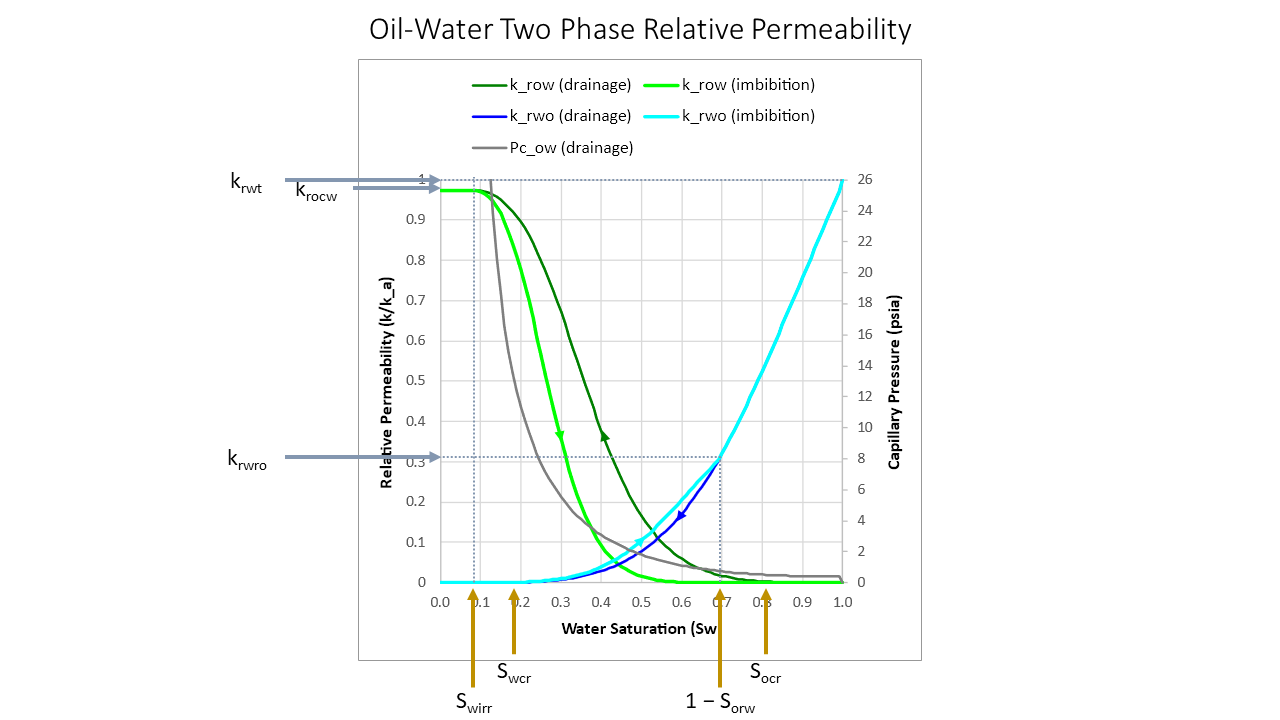
Starting with 100% water saturation (Sw = 1.0) the relative permeability to water is 1.0 and to oil is zero. As the oil saturation increases the oil relative permeability increases and the water relative permeability decreases following the drainage lines until the irreducible water saturation (Swirr) is reached. At this point the relative permeability to oil at the critical water saturation (krocw) is reached and water relative permeability is zero.
Note that oil does not flow until oil saturation is above a small critical oil saturation (Socr). This is not explicitly modelled as the use of LET curves allows some curvature in the lower part of the gas relative permeability curve and the upper part of the oil relative permeability curve which captures this phenomenon. Similarly, the irreducible water saturation, or the minimum water saturation below which water cannot be further reduced, is close to the critical water saturation (Swcr) which is the saturation above which water begins to flow. As with the Socr, this is not explicitly modelled but the use of LET curves allows curvature in the lower part of the water relative permeability curve which captures the phenomenon.
The relative permeability curves exhibit hysteresis, so as water saturation begins to increase again above the critical water saturation (Swcr), an imbibition line is followed. Under circumstances of increasing water saturation, the relative permeability to oil gradually decreases, and the relative permeability to water increases, until the residual oil saturation in the presence of water is reached (Sorw). Note that the relative permeability to water at the residual oil saturation (krwro) is less than 1.0.
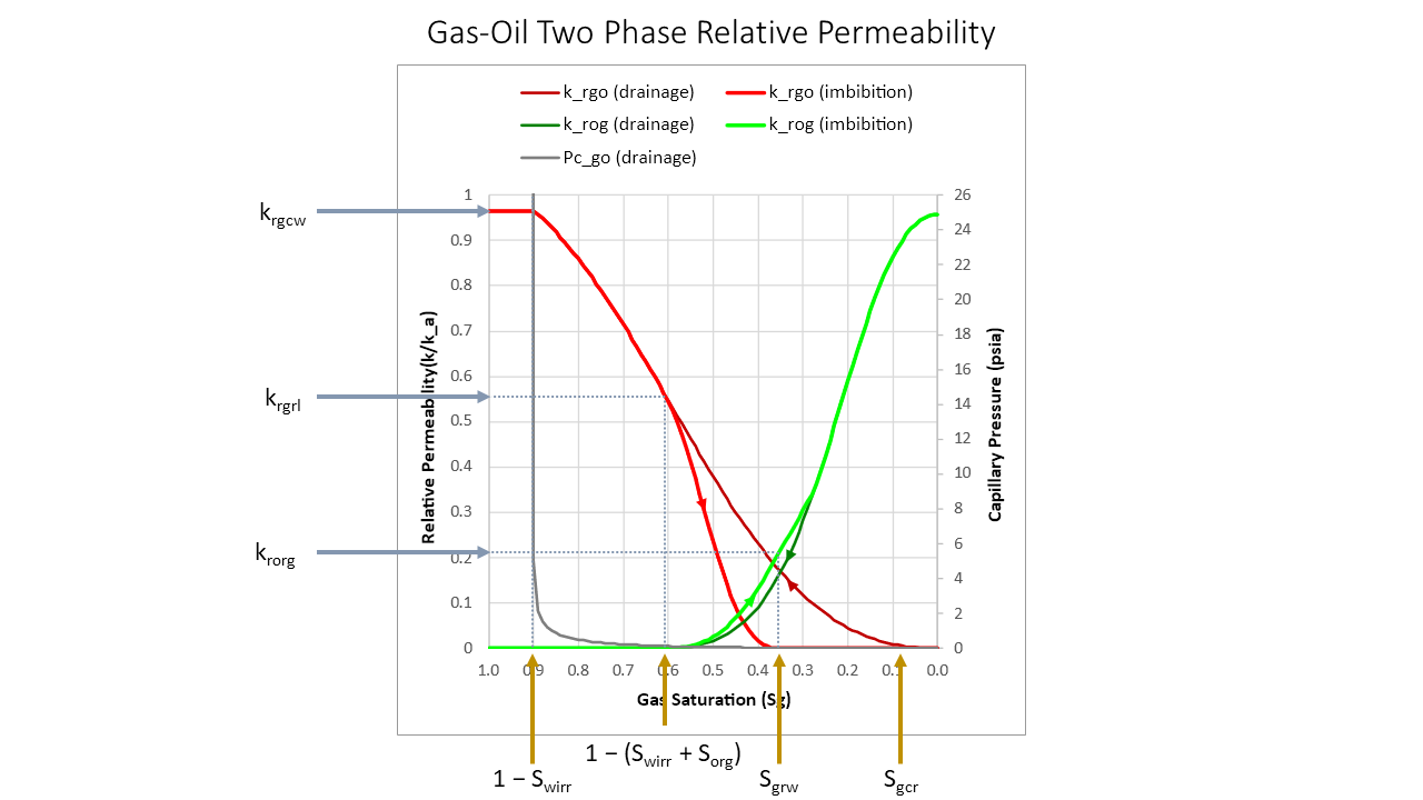
For the gas-oil system, starting with 100% oil saturation the initial relative permeability to gas is zero and to oil is krocw, as gas saturation increases and displaces oil, the relative permeabilities follow their respective drainage curves until the maximum gas saturation allowing for irreducible water and residual oil is reached at 1.0 – (Swirr + Sorg). Whilst this is a two phase relative permeability curve for gas and oil, because reservoir rock will always contain irreducible water, its presence is also considered when calculating the gas saturation. Note that gas does not flow until gas saturation is above a small critical gas saturation (Sgcr). This is not explicitly modelled as the use of LET curves allows some curvature in the lower part of the gas relative permeability curve and the upper part of the oil relative permeability curve which captures this phenomenon.
Since we might also have a situation where there is just gas and water (i.e. no residual oil saturation) an imbibition curve is modelled starting from 1.0 – Swirr. This allows the relative permeability to condensate that is increasing in the reservoir to be captured, with initial relative permeability to gas at the critical water saturation of krgcw decreasing along with gas saturation until the irreducible liquid saturation (irreducible water saturation plus residual oil saturation) is reached with relative permeability to gas of krgrl. As gas saturation decreases below this point, hysteresis is observed up to a minimum gas saturation being the residual gas saturation Sgrw. Note that residual gas saturation in the presence of water is used as this is assumed to be the same as the residual gas saturation in the presence of oil. The relative permeability to oil at the residual gas saturation is krorg.
LET Correlations
Pyrus generates relative permeability curves following the LET method. Use of a LET correlation allows all required relationships and behaviours to be implemented. This is a generalised fitting approach that takes three parameters to control the lower part of the curve (L), the position of elevation of the curve (E) and the upper part or top of the curve (T). Whilst the acronym for the method appears to be an amalgamation of the parts of the curve being modelled e.g. Lower, Elevation and Top, it is more likely that this is actually derived from the author’s surnames being Lomeland, Ebeltoft and Thomas.
Essentially this method works by fitting “S” or “J” curves between specified endpoints. Provided the endpoints can be specified appropriately, then physically reasonable relative permeability curves can be generated. An attractive aspect of this approach is that the generated curves are smoothly continuous over the entire saturation range. In this regard they are considered superior to other common correlations used in industry such as Corey curves.
There are several relative permeability curves in total to account for both drainage and imbibition curves in oil-water and gas-oil systems. For oil-water systems, we must additionally account for water-wet and oil-wet rock. These curves are defined as:
Drainage Oil-Water System
Where:
krow = Oil relative permeability in presence of water, fraction
krwo = Water relative permeability in presence of oil, fraction
krocw = Oil relative permeability at critical water saturation, fraction
krwt = Total water relative permeability, fraction
Se = Effective water saturation, fraction
Swn = Normalised water saturation, fraction
Low = Lower empirical parameter for oil phase with associated water phase, dimensionless
Eow = Elevation empirical parameter for oil phase with associated water phase, dimensionless
Tow = Top empirical parameter for oil phase with associated water phase, dimensionless
Lwo = Lower empirical parameter for water phase with associated oil phase, dimensionless
Ewo = Elevation empirical parameter for water phase with associated oil phase, dimensionless
Two = Top empirical parameter for water phase with associated oil phase, dimensionless
Imbibition Oil-Water System
Where:
krow = Oil relative permeability in presence of water, fraction
krwo = Water relative permeability in presence of oil, fraction
krocw = Oil relative permeability at critical water saturation, fraction
krwro = Water relative permeability at residual oil saturation, fraction
Swn = Normalised water saturation, fraction
Low = Lower empirical parameter for oil phase with associated water phase, dimensionless
Eow = Elevation empirical parameter for oil phase with associated water phase, dimensionless
Tow = Top empirical parameter for oil phase with associated water phase, dimensionless
Lwo = Lower empirical parameter for water phase with associated oil phase, dimensionless
Ewo = Elevation empirical parameter for water phase with associated oil phase, dimensionless
Two = Top empirical parameter for water phase with associated oil phase, dimensionless
For a water-wet system where Swn = 1, then set krwo (imbibition) to krwo (drainage).
Drainage Gas-Oil System
Where:
krgo = Gas relative permeability in presence of oil, fraction
krog = Oil relative permeability in presence of gas, fraction
krocw = Oil relative permeability at critical water saturation, fraction
krgcw = Gas relative permeability at critical water saturation, fraction
Se = Effective water saturation, fraction
Sln = Normalised liquid saturation, fraction
Lgo = Lower empirical parameter for gas phase with associated oil phase, dimensionless
Ego = Elevation empirical parameter for gas phase with associated oil phase, dimensionless
Tgo = Top empirical parameter for gas phase with associated oil phase, dimensionless
Log = Lower empirical parameter for oil phase with associated gas phase, dimensionless
Eog = Elevation empirical parameter for oil phase with associated gas phase, dimensionless
Tog = Top empirical parameter for oil phase with associated gas phase, dimensionless
Imbibition Gas-Oil System
Where:
krgo = Gas relative permeability in presence of oil, fraction
krog = Oil relative permeability in presence of gas, fraction
krgrl = Gas relative permeability at residual liquid saturation, fraction
krorg = Oil relative permeability at residual gas saturation, fraction
Sln’ = Normalised liquid saturation, fraction
Lgo = Lower empirical parameter for gas phase with associated oil phase, dimensionless
Ego = Elevation empirical parameter for gas phase with associated oil phase, dimensionless
Tgo = Top empirical parameter for gas phase with associated oil phase, dimensionless
Log = Lower empirical parameter for oil phase with associated gas phase, dimensionless
Eog = Elevation empirical parameter for oil phase with associated gas phase, dimensionless
Tog = Top empirical parameter for oil phase with associated gas phase, dimensionless
When the water saturation (1.0 minus gas saturation) is less than Swirr + Sorg, then set krgo (imbibition) to krgo (drainage), otherwise use the minimum of the LET equation for krgo (imbibition) and krgo (drainage).
For krog (imbibition) we take the maximum of the LET equation for krog (imbibition), krog (drainage) and krog (drainage) + difference between krog (imbibition) and krog (drainage) ∕ 1.1 at a gas saturation 0.01 higher. This helps the imbibition and drainage curves merge together nicely.
Saturation Inputs
Effective water saturation removes the effect of irreducible water saturation so that effective saturation varies from 0 to 1 between irreducible water saturation and 100% water saturation. Normalised water saturation removes the effect of both irreducible water saturation and residual hydrocarbon saturation, so that normalised saturation varies from 0 to 1 between irreducible water saturation and (1 – residual hydrocarbon saturation).
LET Parameters
The LET empirical parameters have been determined through trial and error experimentation to generate curves that resemble actual core measured data. Whilst these could probably be improved, the basis for modelling the curves is that the endpoints and behaviour of the curves is more critical, and the precise shape of the curves is of second order importance.
| Oil-Water | Water-Oil | Oil-Gas | Gas-Oil | |
|---|---|---|---|---|
| Lower parameter (L) | 1.5 × β | Low | 1.25 + β / 2 × σgo / (0.15 + σgo) | Log |
| Elevation parameter (E) | Low | Low / 2 | Log | MAX(1, Lgo / 2) |
| Top parameter (T) | IF(θow > 90°, 1, 2) | IF(θow > 90°, 2, 0.9) | 1.25 + 0.75 × σgo / (0.15 + σgo) | 1.1 |
Curve Endpoints
First let’s consider the saturation endpoints.
- Swirr or Swcr: This can be obtained from the Holmes-Buckles equation and is related to the pore throat size relationship to the pore size.
- Sgrw: The residual gas saturation after water invasion can be obtained from the Holtz-Land equation. An additional constraint must be considered where the value used cannot be larger than 0.9 × (1.0 − Swirr).
- Sorw: For an oil-wet reservoir with a contact angle θow > 90°, we set the residual oil saturation to the same value calculated for the irreducible water saturation. In other words, if oil is the wetting phase, then it should behave similarly to water as the wetting phase. For a water-wet reservoir, we set the residual oil saturation to the same value as the residual gas saturation subject to an additional constraint where the value used cannot be larger than (1.0 − Sgrw − Swirr) ∕ 1.5.
- Sorg: This is modelled using the Al-Nuaimi equation where Sorg,imm = Sorw. We also consider the additional constraint that the value used cannot be larger than 0.9 − Sgrw − Swirr (or zero if the constraint is less than zero).
Now we can also consider the relative permeability endpoints:
- krocw: Based on krow LET equation for oil-water drainage system at irreducible water saturation. This is equation [A4] in in Lomeland, Ebeltoft and Thomas (2005).
- krwt: Equal to krwro for an oil-wet system or 1.0 otherwise.
- krwro: Based on krwo (water-wet) LET equation for oil-water drainage system at effective saturation = 1.0 − Sorw or zero if this is a negative result.
- krgcw: Based on krgo LET equation for gas-oil drainage system at irreducible water saturation. This is equation [C4] in in Lomeland, Ebeltoft and Thomas (2005).
- krgrl: Based on krgo LET equation for gas-oil drainage system at effective saturation = 1.0 – Sorg.
- krorg: Based on krgo LET equation for gas-oil drainage system at normalised saturation = 1.0 − Sgrw or zero if Sorg + Sgrw + Swirr > 1.0.
These endpoints can be used to construct sets of oil-water and gas-oil two phase relative permeability curves for both drainage and imbibition. The sets of curves generated are consistent with each other. Gas-water curves are not considered separately as conventional simulator inputs only expect a set of oil-water and gas-oil curves. Whilst it is recognised that the gas-water relative permeability curves would be slightly different, the gas curves from the gas-oil system and the water curves from the oil-water system can be combined to create a proxy for a set of gas-water curves.
Relative Permeability Curve Behaviour
Porosity Variation
A consequence of how Pyrus models rock properties is that many parameters can be directly or indirectly linked to porosity. Ultimately the key inputs for Pyrus are the porosity and the nature of the rock fabric. From this are derived permeability, irreducible saturations, residual saturations etc. We should therefore expect a variation in the relative permeability curves to be observed.
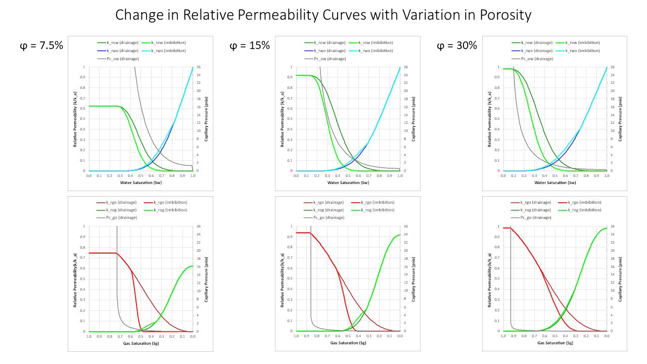
As porosity decreases, the irreducible water saturation increases. This affects the endpoint for the relative permeability to oil at critical water saturation (krocw) and the relative permeability to gas at critical water saturation (krgcw) which both reduce. Note that the LET correlations ensure that the relative permeability curves retain a smooth function and that there are no discontinuities evident as porosity is changed.
Curve Shape
The shape factor β is the same shape factor used for generation of the capillary pressure curves and introduces a consistent basis for a relationship between the capillary pressure curve and the relative permeability curve. Note that the value of is β somewhat arbitrary, although values closer to 1 are consistent with tight, shaley sandstones and values close to 3 are consistent with vuggy carbonate. As with capillary pressure curves, a default value of 2 should perform adequately when generating relative permeability curves.
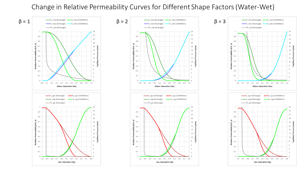
The main difference between the curves as the shape factor increases is that the relative permeability at the point where water or gas flows preferentially to oil is decreased as the shape factor increases. In other words Socr increases as the shape factor increases.
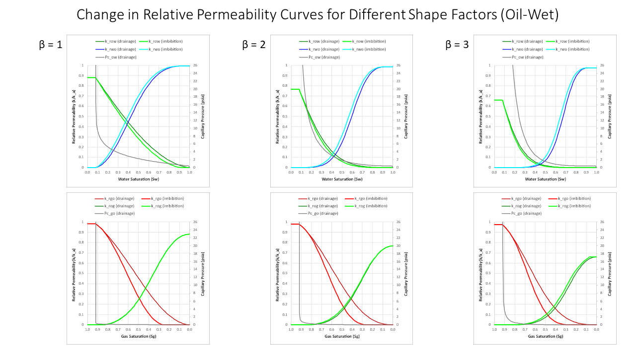
Wettability
A different family of curves is obtained for oil-wet systems. Here oil is the wetting phase and there is less hysteresis apparent between the oil drainage and imbibition curves as a result, and more hysteresis apparent between the water drainage and imbibition curves. No adjustment has been made to the irreducible water saturation for an oil-wet system although this would more likely be similar to residual oil saturation in a water-wet system.
Miscibility
For the gas-oil system, the interfacial tension has an important influence on the relative permeability curves. Under miscible conditions, where interfacial tension decreases (especially lower than 0.1 dyne/cm2), the curves approach an “X” shape with endpoints close to effective saturations of 0.0 and 1.0. At higher IFTs the relative permeabilities exhibit more curvature and the critical oil saturation increases.
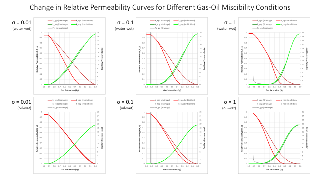
The behaviour of the generated curves is as expected. Note that the oil-water curves are not affected by gas-oil miscibility which is to be expected. As gas and oil become more miscible, the curves lose their curvature and both the critical oil saturation and residual oil saturation decrease. Note that for the water-wet rock, the gas imbibition curve saturation endpoint does not move. This is because the Sgrw (residual gas saturation after water invasion) is used and this value is unaffected by gas-oil miscibility. Since the two-phase relative permeability curve also captures the effect of irreducible water saturation, this is reasonable.
For an oil-wet system a similar approach to that used for Sorg can be employed to generate a value of Sgro that also reduces below a critical IFT of 0.15 dyne/cm2. This eliminates the presence of trapped gas which is an immiscible fluid phenomenon. For an oil-wet reservoir, under miscible conditions the drainage and imbibition relative permeability curves form the idealised “X” shape.