The SEG-Y format is logical when considering the era in which it was devised where tape drives were used for large data storage. Storing data samples sequentially, one trace after the other, means that data can easily be read and manipulated one trace at a time. This limits the need to fast forward and rewind through the tape. With hard drives the limitations still exist to some extent as data is physically stored on tracks which contain sequential data on a platter. However, the ability to move the read head on the drive across different tracks means that seeking to the end of a file is considerably faster than where all data is stored on a sequence of reels of magnetic tape. With modern solid state drives all moving parts have been eliminated. This not only enhances the reliability of the storage medium but also means that the physical limitations that have constrained large data structures are no longer necessarily a concern.
Understanding What Makes Read Access Slow
A few years ago it occurred to me that there might be a better way to structure the data on a file so as to optimise the read time for different planes of data through a 3D volume. In particular, to speed up the reading of slices by trading off a small increase in read time for the inlines. Initially I didn’t know whether this would be possible or not and there was no compelling business need to investigate. It was something of a challenge to set myself and along the way perhaps I would learn something useful?
Where does one start when trying to determine whether it is possible to improve read speeds of large datasets? One might imagine that this is not a new challenge to confront many different industries using large data. Almost certainly there probably exists a solution that was ready to apply to the problem. Rather than immediately looking for the answer I spent some time thinking about how data is physically read from a storage medium. What is it that makes the reading of a slice so much slower than an inline? After all, for many volumes a slice contains fewer samples than an inline, so if an equal time were spent reading each sample then reading a slice should be faster. The fact that it is much slower suggests that reading of sequential bytes is much faster than skipping bytes and reading one at a time.
This certainly makes physical sense when you consider how data is stored on the platter of a hard drive. Magnetic information is recorded onto the surface of a platter. As illustrated in Figure 1, this data is laid out in tracks so that sequential byte streams pass under the read head of the drive as it rotates. Data is accessed at the speed that the drive spins i.e. a 10,000 rpm drive will have a faster sequential read speed in comparison to a 5,400 rpm drive. To access non-contiguous data the read head must traverse across the platter to a different track and/or the platter must rotate to the position of the data on that track. The seek action has a latency associated with this physical movement which is much slower than the time between reading of consecutive bytes on a track. Therefore reading data that is stored in a contiguous fashion is much faster than reading the same volume of data if it is stored sparsely.
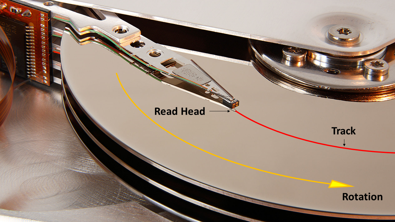
Source: Wikipedia
So let’s think about what happens when we read a plane of data from a 3D volume. Ultimately a file is a one-dimensional sequence of ‘1’s and ‘0’s. These binary numbers are assembled into bytes (eight bits per byte) and a sequence of bytes can be used to represent different data types. For example four bytes can be used to represent a floating point number. Even though the data represents a three dimensional volume, a one dimensional offset is needed to get the sample value at a given location. For example, in a data volume of single-precision floating point numbers 100 x 100 x 100 in size, I might request the data sample at location 10, 10, 10. If the data is structured similar to SEG-Y e.g. data is recorded sequentially in the z-direction, then the y-direction and finally the x-direction, we can calculate the byte offset for this data sample. To get to the data sample I would first need to skip over nine inlines (each containing 100 x 100 samples), then skip over nine traces (each containing 100 samples) and finally skip over nine samples. The very next byte, at byte offset 363636, will be the first of four bytes representing our floating point number. If we think about how the data is physically stored on the hard drive, to get to byte offset 363636 it is necessary to move the read head over to the correct track and then allow the spinning platter to rotate and line up with that location. All of this takes a fixed amount of time, whether I then go on to read just a single byte, floating point number or indeed an array of bytes.
Interestingly the same principle applies to solid state drives. Contiguous data has a much faster access speed than randomly stored data. This is due to the latency inherent between issuing a read request and the response time for the controller and software on the device to access the specific data location and return the result. In comparison to RAM, which has a latency of 0.04 to 0.1 μs, the read latency of NAND flash varies from 25 μs for single-level cells (SLC) to 100 μs for triple-level cells (TLC). This is thousands of times slower. Without going into detail, the important aspect to note is that any strategy devised for speeding up read access on hard drives should apply to solid state drives too.
Towards a More Efficient Data Structure - Chunking
Writing software to optimally take advantage of hardware capabilities is sometimes referred to as mechanical sympathy. Essentially the software needs to work in harmony with the capabilities of the hardware so as to eke out the maximum potential performance. In the case of reading a slice from a SEG-Y volume, the software is quite literally getting in the way of the hardware. The fact that it can be done today with faster hardware than was available 20 to 30 years ago does not mean we should not try to implement a better solution. I share the bewilderment that as hardware continues to advance, sometimes software appears to move in the opposite direction. Perhaps it is because of their very versatility that computers can be shoehorned to fulfil almost any task, and as long as their performance continues to increase, no-one will really notice that cat videos do not actually require the latest and greatest hardware. In my case though a computer still needs to meet its basic function; it must be able to compute… fast.
If we look at the read times for different SEG-Y lines on a hard drive we see that the inlines are an order of magnitude faster than a crossline and several orders of magnitude faster than a slice. Testing on a 3D post-stack seismic volume with dimensions 1,966 x 1,103 x 3,001 we find the following results:
| Metric | Sample Read Time (μs/float) | Line Read Time (sec) | Time Factor vs Inline (x) |
|---|---|---|---|
| Inline | 0.064 | 0.2 | 1.0 |
| Crossline | 1.1 | 6.6 | 17.5 |
| Slice | 150 | 320 | 2,270 |
In effect it would be possible to read many inlines in the time that it takes to read a single crossline (33x slower) or slice (1,600x slower). This is the power of contiguous data: it can be read incredibly fast.
The kernel behind any solution must therefore be one where irrespective of the plane of data required, the number of seeks or skips through the dataset is minimised and most of the data can be read using sequential reads. One such structure to achieve this outcome would be if the volume were to be split into several smaller volumes or cubes. Each sub-volume would store its data contiguously, and the sub-volumes are arranged such that they can be formed into slabs that encompass inlines, crosslines and slices. An example of this structure is illustrated in Figure 2.
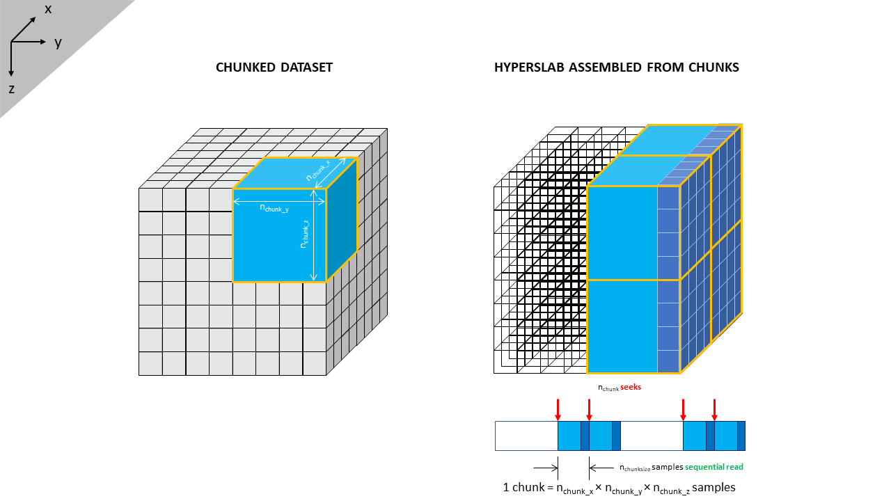
This illustrates a very basic data volume 8 x 8 x 8 in size. Without any sub-volumes, to read a crossline would require eight seeks in total, plus eight sequential reads of eight samples each. Instead let’s break the volume up into eight sub-volumes or ‘chunks’ each of which contains 4 x 4 x 4 = 64 samples. Each chunk can be read contiguously and parts of the chunks can then be re-assembled into a crossline. This alters the reading of a crossline to four seeks in total, plus four sequential reads of 64 samples each, followed by discarding of 192 redundant samples. At first glance this appears grossly inefficient as we are reading a large volume of data that is then discarded as redundant. Why bother reading it in the first place? However, we have halved the number of seeks.
Using the stated specifications for each drive in addition to the Intel Optane 800p published specifications we can calculate the theoretical expected time for reading a crossline in a standard volume and in a chunked volume:
| Metric | Hard Drive | SATA III SSD | NVMe SSD | Optane |
|---|---|---|---|---|
| IOPS (QD1) | 118 | 12,000 | 14,000 | 55,000 |
| Seek time / latency (μs) | 8,500 | 83.3 | 71.4 | 18.2 |
| Data rate (Mbit/s) | 1,030 | 4,420 | 28,000 | 11,600 |
| Data rate (Mbyte/s) | 128.75 | 530 | 3,500 | 1,450 |
| Read time (ns) | 7.8 | 1.9 | 0.3 | 0.7 |
If we define time for a seek as ‘t_s’ and time to read a sequential byte as ‘t_b’, with a chunk size of ‘n_chunk_x’ x ‘n_chunk_y’ x ‘n_chunk_z’, then the time to read the crossline in a standard volume is:
Time to read the crossline in a chunked volume is:
Applying these equations to the theoretical drive speeds leads to the following times:
| Metric | Hard Drive | SATA III SSD | NVMe SSD | Optane |
|---|---|---|---|---|
| Unchunked Time (μs) | 68,000.5 | 666.5 | 571.2 | 145.6 |
| Chunked Time (μs) | 34,002 | 333.7 | 285.7 | 72.9 |
| Speed-up Factor | 2.0x | 2.0x | 2.0x | 2.0x |
In this particular example the total read time is dominated by the seek times. Halving the number of seeks halves the total read time e.g. a speed-up factor of double. Indeed, the whole example is a little contrived since it would be faster to just have a single chunk comprising the entire volume and to read this in its entirety, thus only requiring a single seek. In the real world the data volumes are of course much larger and there should be a crossover point where the chunks become so large, and contain so much redundant data to be discarded, that the sequential read time exceeds any benefit from reducing the number of seeks.
To illustrate the theoretical advantage of chunking, we can plot the average read time for an inline, crossline and slice against the chunk dimension for different storage media using our equations. This is shown in Figure 3.
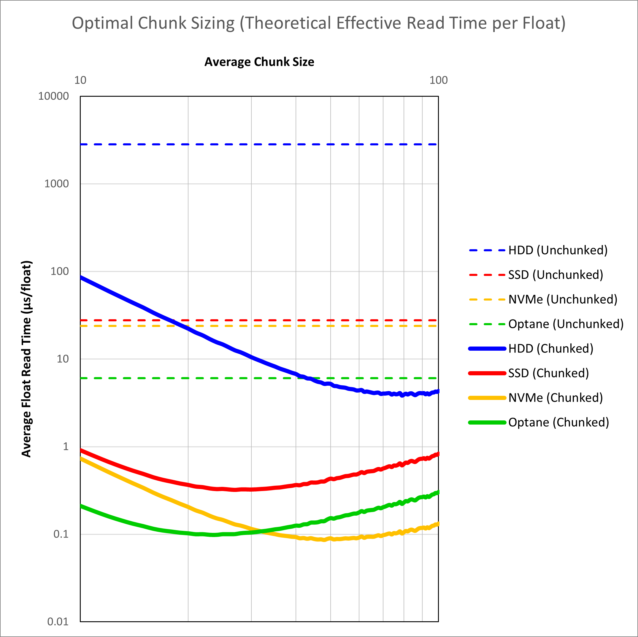
We see that when dealing with unchunked volumes, improving the hardware alone leads to gains. The combination of hardware and chunking delivers the best results. It is interesting to note that with chunking alone, even a hard disk drive should be able to exceed the performance of an unchunked volume on Optane. Optane itself is also not a clear winner. A fast NVMe solid state drive should be able to match Optane as a result of the very fast sequential read speeds on these drives. Overall the speed improvement from application of chunking should be over two orders of magnitude faster, and potentially less than 0.1 μs per float. This is a critical value as less than 0.1 μs per float starts to approach the inline read speed for a conventional SEG-Y volume (0.064 μs per float for a hard drive to 0.017 μs per float for a NVMe SSD).
Don’t Reinvent the Wheel - Hierarchical Data Format
Having in theory found a potential solution to speed up average data access for large 3D volumes, the next challenge is to implement it. Whilst it is always possible to implement a custom solution, a better approach is to utilise an established format which is well documented and tested.
Whilst it would be great to think that I had invented an innovative or unique approach to reading SEG-Y data, the reality is that there are many industries and scientific fields that must also deal with large data sets. Before the current “artificial intelligence” buzzphrase, “big data” was all the rage. Thankfully business’ enamourment with big data has meant that a great deal of resources have been devoted to the topic. The approach of ‘chunking’, it turns out, is not new – I merely happened to have independently discovered this approach that has widespread acceptance across numerous disciplines. Because of the many different needs for a solution, there exists a standard file format that was designed with chunking in mind. This is the HDF5 hierarchical data format.
An attraction of HDF5 is that it is a defined format that implements a versatile data model. The data model is general and allows for a variety of different data types to be stored in an unlimited file size, yet the data volume can be expanded or contracted without compromising access speed. Perhaps the biggest attraction is that there are a number of software libraries which facilitate manipulation of the file format. Thus adoption of HDF5 means that the programmer can focus on the implementation of the data model rather than worrying about the nitty-gritty of file access.
As a test, the 1,966 x 1,103 x 3,001 SEG-Y seismic volume was converted to HDF5 format using different chunk sizes. A benchmark was created to read random inlines, crosslines and slices from the SEG-Y and chunked HDF5 volumes. The average read times for these different permutations are shown in Figure 4.
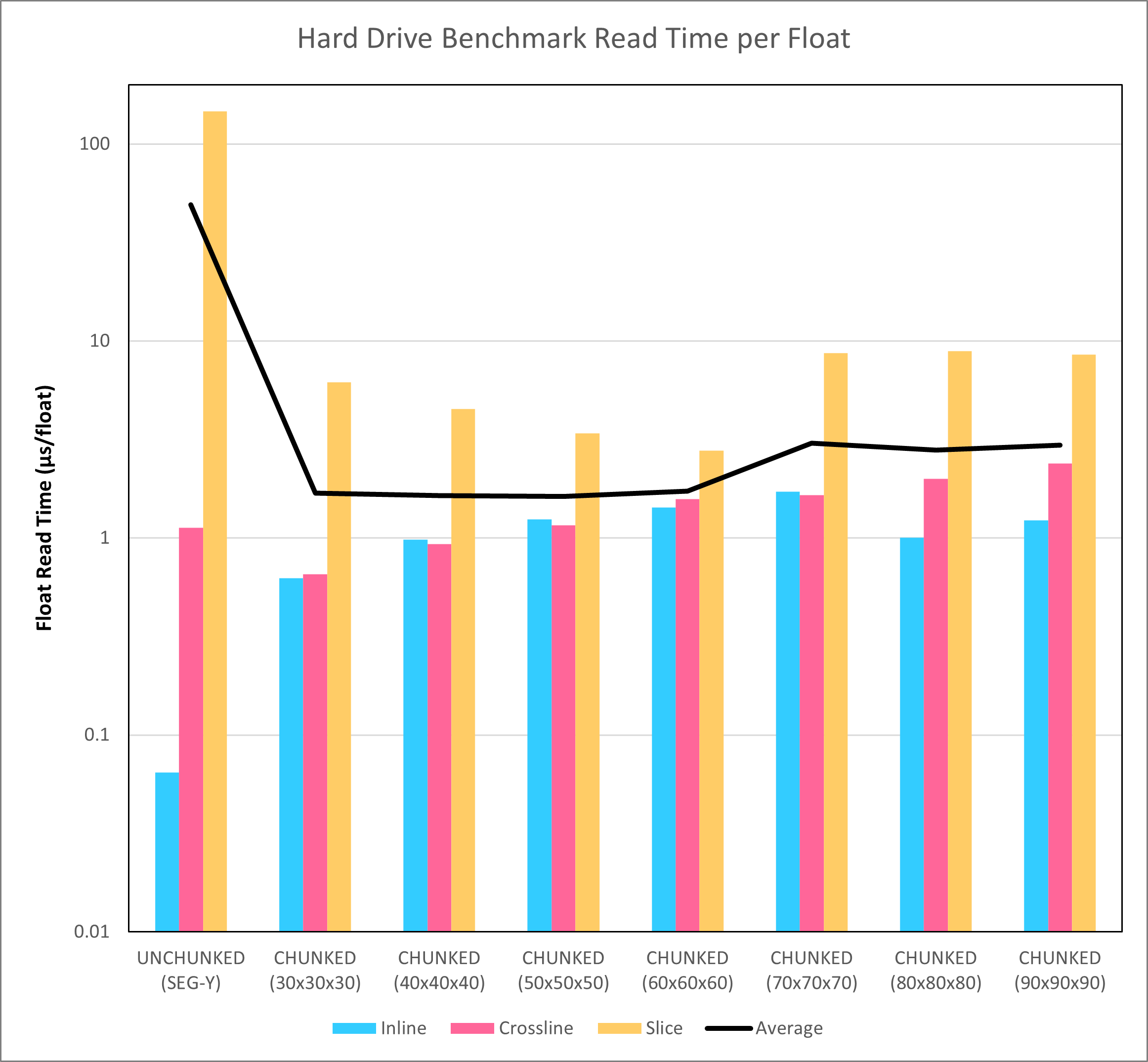
The HDF5 chunked format offers much more consistent access to data, irrespective of the planar type requested. Whereas there is a difference in read speed that is several orders of magnitude apart with the SEG-Y format, for the HDF5 format there are only minor differences apparent between access for an inline versus a crossline or slice. Furthermore, the average read time is improved by more than an order of magnitude. Given that this is nothing more than just a restructuring of the data stored in the file, this is a huge win.
What should also be noted is that the actual read times for the hard disk drive do not match up well with the theoretical times shown in Figure 3. It was noted during an earlier examination of SEG-Y read times that the hard disk drive buffer helps to reduce the effective latency associated with seeks that are not too far apart in the file. Therefore the measured times for the hard disk drive are lower than the theoretical times. It is also interesting that the theoretical times predicted that the best performance would be achieved with larger chunk sizes (dimensions 70 to 90). Actual performance appears to be somewhat agnostic towards the chunk size, perhaps because of differences in how the buffer is affecting the results for different chunk sizes. Whether this also applies to results obtained with solid state drives will be examined in a later blog post.
Is Chunking Worth It?
On the basis of consistent read time alone, the answer would have to be a resounding yes. Yet ‘HDF5’ and ‘chunking’ are not common terms used in the oil and gas industry. There has been some adoption, but it is far from widespread. This begs the question, “if HDF5 and chunking is really that good, surely everyone would be using it?”.
Fundamentally there are two costs associated with chunking.
- The original data volume must be copied and restructured into a chunked volume. This takes time. Whilst not excessive it means that the volumes must be prepared prior to use of the chunking strategy. There are also legacy data issues. For a single newly acquired volume, this might not be such a burden. However, consider a company with a large database of 3D data that runs to many terabytes or more. Converting all the data to a new format will be costly: time, resources to manage the conversion and the additional storage space needed for the converted volumes. Furthermore, there is a large legacy of software programs that use the data – most of which cannot read the HDF5 format.
- Inline read speeds are slower than an unchunked volume. There is no getting around this. For the absolute fastest speeds an unchunked volume will always give the best inline read speeds. However, this alternative strategy requires a dedicated volume for inlines, crosslines and slices. If an arb-line (random line across the volume) is needed, the speed will be just as slow as a typical crossline whereas the chunked approach will deliver the same speed advantages even if the data requested is not orthogonal.
In that context the industry mantra is probably one of, “if it ain’t broke, don’t fix it”. My conclusion is that as an internal format for seismic data in the Pyrus Suite, the use of HDF5 is a no-brainer. It is more robust, simpler and faster than SEG-Y. Having discovered chunking and its benefits, the next challenge is to implement it into the Pyrus Suite.