After deciding to adopt chunking with the HDF5 format for the Pyrus program, it is advantageous to consider whether the implementation has been optimised. The whole point of using HDF5 is to improve the performance of data reads in comparison to the conventional SEG-Y format, so we don’t want to leave any potential performance gains on the table. In this article we will consider the performance of the jHDF library and how to balance the read times for inlines, crosslines and slices. Comparison of different HDF5 libraries showed that jHDF could deliver the fastest read speeds when used with large chunks and a parallel algorithm. As this is coded in Java and is a open source project, it means that we can delve into the code and examine if it is possible to improve its performance. We also consider the chunk shape itself; will a squashed cuboid permit faster access for the slow directions (crossline and slice) by optimising the number of sequential byte reads along those directions in a chunk?
Optimising IO in Java
When looking at the performance of jHDF against various chunk sizes, it is apparent that the smaller chunk sizes do not perform as well. This does not appear to be a hardware limitation as the native HDF library is able to comfortably outperform the jHDF library. One difference between the two approaches is that the jHDF implementation used was reading chunks in parallel. It is known that thread instantiation carries some overhead, and it is possible that using a large number of threads for smaller chunks could be leading to poor performance? This was unlikely as in the benchmark the number of threads was deliberately limited to 16 (AMD Ryzen 7 1700 CPU with eight cores and two threads per core). Each thread was reused once reading of a chunk completed, thus there was no unnecessary thread creation. Nonetheless, to test whether the parallel algorithm was the source of the problem at lower chunk sizes, the benchmark was repeated with a single threaded implementation of the jHDF library. The results are shown in Figure 1.
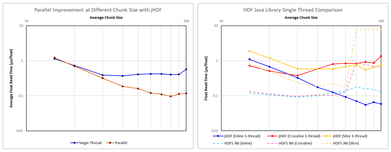
It can be seen that at smaller chunk sizes the performance of the single-threaded implementation and the parallel implementation are essentially identical. Therefore we can rule out problems with the parallel code as a cause for the poor performance.
Also shown in Figure 1 is the performance of the single-threaded jHDF implementation for inlines, crosslines and slices against the native HDF library. There is a remarkable difference in the read speeds for both inlines and crosslines for small chunk sizes between jHDF and the native HDF library. If access to the hardware is limited by the same physical (electronic) constraints, then the native library should, in theory, be slower because of the overhead associated with wrapping the native code. However, it is significantly faster. Furthermore, where with jHDF the performance for crosslines diverges from inlines at chunk sizes above 30x30x30, with HDF5 JNI the inline and crossline performance is similarly fast. This is counter-intuitive as we would anticipate that the crossline reads are slower. To understand what is happening, we need to look at the source code for jHDF, and in particular the io.jhdf.api.dataset.ChunkedDataset.getRawChunkBuffer() method.
There are two main libraries for IO in Java. These are java.io.* and java.nio.*. Java IO effectively wraps the operating system native IO methods such that the JVM provides an OS-independent interface to file operations. This provides all the benefits of the strongly typed Java language at the cost of some overhead. Java New IO (NIO) provides methods for accessing raw bytes stored in non-heap memory through a ByteBuffer. This enables fast random access to large byte arrays. To create a ByteBuffer using Java NIO, there are two principle approaches that can be used. My understanding of the differences between the two methods is summarised as follows:
- Wrap a Byte Array: The byte array is created on the JVM heap and provides a backing array to the ByteBuffer. Because the data is read into the JVM heap, there are no array copies required.
File infile = new File("/path/to/file");
long address = 0L; // byte offset position in file to read from
FileChannel fc = new RandomAccessFile(infile, "r").getChannel();
byte[] b_array = new byte[n_bytes];
ByteBuffer bb = ByteBuffer.wrap(b_array);
fc.read(bb, address);
- Memory-mapped ByteBuffer: Memory map the
ByteBufferusing non-heap memory to the underlyingFileChannel. This can provide a performance boost if the data being mapped already resides in memory as a result of being previously read. In addition, only data that needs to be copied into heap memory for the byte array is copied, in contrast to the wrapped byte array where the entire buffer is read into the heap.
File infile = new File("/path/to/file");
long address = 0L; // byte offset position in file to read from
FileChannel fc = new RandomAccessFile(infile, "r").getChannel();
byte[] b_array = new byte[n_bytes];
ByteBuffer bb = fc.map(MapMode.READ_ONLY, address, n_bytes);
bb.get(b_array);
Comparison testing between the two methods using random reads on a large multi gigabyte file suggests that the wrapped approach is slightly faster both for single-threaded and parallel implementations. However, when applied to the reading of chunks from an HDF5 file, the wrapped approach exhibited no speed benefit from parallel versus single-thread and the mapped approach was overall faster. The reasons for this are not clear.
For the moment it would appear that the jHDF implementation is using the fastest access method for file IO.
There is definitely raw performance to be gained as indicated by the superior performance of the HDF5 JNI library for small chunk sizes. For the moment we will remain satisfied that superior performance with larger chunk sizes is attainable ‘‘as is’’ with the jHDF library and move onto balancing the read times for inlines, crosslines and slices.
Optimising Chunk Shape to Balance Read Times
So far all benchmarking has reorganised the SEG-Y file into a chunked HDF5 format using perfect cube chunks. For the initial benchmarking this was an appropriate strategy as it removed any variability that could arise as a result of non-symmetric chunk shapes. Having determined that larger chunk sizes (~80x80x80) are optimal, the next stage is to determine if it is possible to balance the read times for inlines, crosslines and slices.
When reading chunks for crosslines and slices, all the bytes in the chunk are read with a large percentage of those bytes read being discarded as redundant. By altering the chunk dimensions to favour a longer crossline direction and a flatter shape (parallel to a slice) the number of redundant bytes for each crossline and slice is reduced. The trick is to define an algorithm that will calculate good chunk dimensions for any 3D volume size as it is doubtful there exists a ‘one size fits all’ chunk shape. This is because the chunk shape needs to consider not only the balance between read speeds in each orthogonal direction, but also the number of chunks that need to be read along a given axis. For example if a volume is very elongated, then the chunks will also need to be elongated to balance the number of chunks read in the long direction versus the shorter directions.
The algorithm proposed is as follows:
- Chunk Size: Divides the seismic volume into an equal number of chunks along each axis, where the chunk has a target number of bytes. The target number of bytes is determined based on the optimal size taking into consideration the hardware latency, sequential read times and parallel read optimisation.
- Chunk Ratio: Chunk dimensions are manipulated by first squashing the chunk to reduce the size in the z-direction and increase along the x-direction and y-direction, whilst preserving the approximate number of bytes. This increases the number of samples per slice read with each chunk, thus improving the efficiency for reading slices.
- Chunk Asymmetry: Inline and crossline read times are then balanced by changing the relative lengths of the x-direction and y-direction. Since inline reads are comparatively fast, a short inline dimension (which leads to an increased number of seeks and thus higher latency) is an acceptable tradeoff for increasing the number of samples per crossline read with each chunk, which improves the efficiency of reading crosslines.
// Calculate the chunk sizing to use
long num_samples = (long) nx * (long) ny * (long) nz;
double target_chunkbytes = chunk_kb * 1024.0;
double num_chunks = Math.ceil(num_samples / (target_chunkbytes / 4.0));
double chunk_dim = Math.ceil(Math.pow(num_chunks, 1.0 / 3.0));
double chunk_x = nx / chunk_dim;
double chunk_y = ny / chunk_dim;
double chunk_z = nz / chunk_dim;
chunk_x = Math.floor(chunk_x * Math.sqrt(chunkratio) * chunkasym);
chunk_y = Math.floor(chunk_y * Math.sqrt(chunkratio) / chunkasym);
chunk_z = Math.floor(chunk_z / chunkratio);
The influence of chunk size, chunk ratio and chunk asymmetry can be seen in Figure 2. This figure shows the actual read time for an inline, crossline and slice (plus the average). Where we have previously only considered the read time per float, this approach now also takes into account the number of floats that need to be read for each plane. This means that a slightly slower read time is OK if there are not as many samples that need to be read for a given plane.
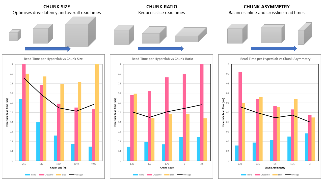
We find that the optimal chunk size is ~2 MB (2,048 KB). This corresponds to an average chunk dimension of ~77 which is close to the 80 x 80 x 80 chunk size that was previously found to be the fastest size for reading with the jHDF library. For a selected chunk size of 2 MB, a higher chunk ratio leads to a reduced slice read time at the expense of increased inline and crossline read times. At first glance it appears that a chunk ratio of 1.5x is optimal. Finally the chunk asymmetry clearly balances the inline and crossline read times.
After some experimentation a chunk size of 2,048 KB, chunk ratio of 2.0x and chunk asymmetry of 2.5x was found to be optimal.
| Plane | Sample Read Time (μs/float) | Number Samples | Line Read Time (sec) |
|---|---|---|---|
| Inline | 0.129 | 3,310,103 | 0.43 |
| Crossline | 0.072 | 5,899,966 | 0.43 |
| Slice | 0.195 | 2,168,498 | 0.42 |
| Average | 0.13 | 0.43 |
Overall this is a satisfactory performance. A sub-half second read time for all lines is achieved. In comparison, reading a slice with SEG-Y format varies from 317 seconds (over 5 minutes!) on a hard drive to to 135 seconds (still over 2 minutes) on an NVMe solid state drive. Of course inline performance suffers, as the chunked file structure is not as fast as reading sequential data. Crossline speeds are similar. A comparison between SEG-Y versus our optimised HDF5 for NVMe SSD hardware is tabulated below:
| Plane | SEG-Y on NVMe SSD (sec) | HDF5 on NVMe SSD (sec) | Speed-up Factor |
|---|---|---|---|
| Inline | 0.06 | 0.43 | 0.15x |
| Crossline | 0.45 | 0.43 | 1.05x |
| Slice | 134.97 | 0.42 | 321x |
| Average | 45.16 | 0.43 | 105x |
Read performance on average is over one hundred times faster than using the SEG-Y format only.
Incidentally similar performance can be achieved with a 40 x 40 x 40 chunk size using the HDF5 JNI library. Also, as previously noted, the fastest performance possible could be obtained by re-writing the entire volume three times so that inlines, crosslines and slices are all in the fast direction, and the storing all three volumes in memory using a RAM disk. This would blitz the solution provided here – although a RAM disk could also be used with the HDF5 file…