Hydrocarbon fluids are mixtures comprising a number of different components. Depending on the environmental conditions that the fluid is subject to, that fluid can be either in a gaseous or liquid state, or comprising both liquid and vapour phases each of which has a different composition. As the fluid phase state, pressure and temperature change, the properties of that fluid also change. Understanding the relationship between the fluid phases and its properties in response to changes in pressure, volume and temperature (PVT) is a crucial activity when building a reservoir simulation.
In a simulator we generally want to know three different properties:
- Density: The mass of a fluid relative to its volume. Fluid density (ρ) governs the pressure profile within a reservoir, including capillary pressures which in turn control the fluid saturations.
- Formation Volume Factor: Also known as FVF this is the relationship between the volume of a fluid at reservoir conditions in comparison to standard conditions (~14.65 psia and 60 °F). This translates the volume of fluid contained within a reservoir pore volume into those at surface conditions which are typically used for measurement of sales volumes.
- Viscosity: This governs how easily a fluid will flow. Viscosity (μ) is an input variable to Darcy’s Law.
It is possible to calculate each of these properties for a fluid at every time step and for each cell in a reservoir. Indeed this is how a fully compositional simulator operates, with the fluid properties for at each time-step and in each reservoir cell determined according to a ‘flash’ calculation. In a modified black-oil simulation approach, given that many cells will have similar pressure and temperature for a consistent composition, the variation in properties can be expected to be linear and smooth as pressure varies. This means that usually the fluid property values are pre-calculated and provided to the simulator in the form of PVT look-up tables (LUT) over the pressure range of interest at reservoir temperature. In addition, the gas density at standard conditions must be supplied in order to calculate the gas FVF at any pressure.
For calculation of PVT tables we can either use correlations or an equation of state. Whilst correlations are useful for quick hand calculations, with the power of a computer available it makes more sense to use the more involved equation of state approach as this allows properties of arbitrary mixtures to be determined with relative ease.
Reservoir Fluid Types
Fluids fall into three different classes. These are incompressible fluids, slightly compressible fluids and compressible fluids. The behaviour of each of these types of fluids is different in a simulator.
Incompressible Fluid
This is an idealised fluid that can be used to represent dead oil (e.g. no solution gas) and water. An incompressible fluid has zero compressibility. A consequence of this is that irrespective of pressure, the density, FVF and viscosity are constant. Mathematically:
Slightly Compressible Fluid
A slightly compressible fluid has a small but constant compressibility (c)that usually ranges from 10−5 to 10−6 psi−1. Gas-free oil, water and oil above bubble-point pressure are examples of slightly compressible fluids. The pressure dependence of the density, FVF and viscosity are expressed as:
Where:
ρo = Fluid density at reference pressure (Po) and reservoir temperature, lbm/ft3
Bo = FVF at reference pressure (Po) and reservoir temperature, rb/stb
μo = Viscosity at reference pressure (Po) and reservoir temperature, cp
cμ = The fractional change of viscosity with pressure change (viscosibility)
Oil above its bubble-point pressure can be treated as slightly compressible fluid with the reference pressure being the oil bubble-point pressure and, in this case, ρo, Bo, and μo are obtained from oil-saturated properties at the oil bubble-point pressure.
Compressible Fluid
A compressible fluid has orders of magnitude higher compressibility than that of a slightly compressible fluid, usually 10−2 to 10−4 psi−1 depending on pressure. The density and viscosity of a compressible fluid increase as pressure increases but tend to level off at high pressures. The FVF decreases orders of magnitude as the pressure increases from atmospheric pressure to high pressure. Natural gas is a good example of a compressible fluid. The pressure dependencies of the density, FVF and viscosity of natural gas are expressed as:
The volume conversion factor is αc = 5.6145835124493 which is the number of cubic feet in one barrel.
Bg is usually stated in units of rb/Mscf.
Alternatively, the gas expansion factor (GEF) can be used. This uses the more intuitive units scf/rcf (or sm3/m3) and is defined as 1 / αc·Bg.
Equation of State
Fluid samples obtained from the reservoir can have their properties measured and analysed in a laboratory. Acquiring fluid samples, especially downhole samples which are more representative of the actual unaltered reservoir fluid, can be both technically challenging and expensive. Even where fluid samples are available, it is not unusual to discover that different samples obtained from the same part of the reservoir can exhibit different properties. Sometimes no laboratory measurement of properties is available, but a compositional analysis obtained using chromatography has been performed.
Using the composition and knowledge of chemistry and physics, the properties for a given fluid under specific conditions can be predicted using an equation of state (EoS). This is an algorithm that predicts for a given pressure and temperature what the associated phase and volume for the liquid and vapour compositions that make up the original fluid are.
The first progress towards understanding the behaviour of fluids was Boyle’s Law as early as 1662 and is recognised as perhaps the earliest basic form of an equation of state. This established that the volume of a gas is inversely proportional to its pressure. The next advance came over 100 years later in 1787 with Charles’ Law which states the volume of a gas is proportional to its temperature under conditions of constant pressure (isobaric).
In 1934 Clapeyron was the first to combine both these laws into a single relationship, the ideal gas law, via the universal gas constant. For an ideal gas the pressure, volume and temperature are related to each other by the ideal gas law. At constant temperature, the pressure multiplied by the volume of the gas should remain constant, and for a constant pressure, as temperature increases the volume of the gas should expand.
Where:
P = pressure
V = volume
T = temperature
n = amount of substance, mol
R = universal gas constant
For a constant temperature, the value nRT is constant and thus the equation indicates that pressure is inversely proportional to the volume. This is Boyle’s Law. Similarly, for a constant pressure the value nR/P is a constant and volume is proportional to temperature. This is Charles’ Law.
In reality, ideal gases do not exist although for many gas mixtures this behaviour can be assumed up to pressure of about 4 bar (60 psia). As pressure increases above this level the accuracy of the relationship decreases. Therefore, for real gases a correction factor z, also referred to as the gas-deviation factor, is introduced:
Cubic EoS
To model gas behaviour the use of a cubic equation of state is commonly applied. In the cubic EoS the gas deviation factor is solved by an equation of the form:
The constants A0, A1, A2 are functions of pressure, temperature, and phase composition.
The first cubic EoS was proposed by van der Waals in 1873. This modifies the real gas equation as follows:
Where:
Vm = Molar volume, the volume of one mole of gas or liquid = V / n
The modifications to the ideal gas law are two-fold and address the neglect of molecular size and intermolecular forces in the ideal gas law:
- It is conceptualised that molecules occupy a small volume and are not infinitessimal small points. Therefore there is an adjustment ‘b’ to the volume applied to subtract the space occupied by the molecules themselves. This parameter is often referred to as the co-volume and is included in a “repulsion” term since it reflects a physical reasoning that molecules will repulse each other if they are too close – this is the behaviour of an incompressible liquid.
- Unlike in an ideal gas, molecules within a real gas will exert an attractive force on each other. This phenomenon manifests itself as a reduction in the pressure on the outer surface of a gas volume. Thus the effective pressure applicable to the ideal gas law is is increased by adding an “attractive” term = a / Vm2 where ‘a’ is referred to as the energetic parameter.
For both the repulsive and attractive modifications, at high temperature and low pressure, where molecules in the gas are further apart and thus the gas has a large molecular volume, we note that (Vm - b) ≈ Vm since Vm » b, and (a / Vm2) ≈ 0. Therefore the equation reduces to the ideal gas law.
Re-arranging gives the form:
In this form of the equation, the first term improves prediction of liquid behaviour since the volume approaches a limiting value of b at high pressures. This term represents the repulsive component of pressure on a molecular scale. The second term accounts for the non-ideal behaviour of the gas and is traditionally interpreted as the attractive component of pressure.
The energetic parameter ‘a’ in the attractive term and the co-volume ‘b’ in the repulsion term are defined as:
Using reduced state variables, Vr = Vm / Vc, Pr = P / Pc and Tr = T / Tc, the van der Waals equation can be written:
This is a cubic equation which has three roots. The largest and the lowest roots are the gas and liquid reduced volumes.
Almost all other cubic EoS follow a similar form to the original van der Waals equation and conceptually they function in a similar manner. The van der Waals equation is no longer used as other cubic EoS are more accurate, but the principles upon which the equation was developed are still relevant and worth understanding. So important were the concepts introduced that Johannes Diderik van der Waals was awarded the Nobel prize in Physics 1910.
Peng-Robinson EoS
There have been many variations proposed and modifications to the basic cubic EoS. Redlich and Kwong (RK), working for Shell, introduced a temperature dependence to the attractive parameter ‘a’ in 1949. After the acentric factor was proposed by Pitzer in 1955 to account for the non-sphericity of molecules and was shown to be related to vapour pressure, it wasn’t until 1972 that Soave modified the RK equation to introduce the acentric factor so that the attractive parameter ‘a’ is a function of both temperature and acentric factor. This gives the Soave-Redlich-Kwong (SRK) form for the cubic equation. The ability of the SRK equation to predict fluid properties led to its popular adoption during a period when computers were also becoming more widespread and which greatly improved the practicality of the equation’s usage.
A recognised shortcoming of the SRK equation is that the critical compressibility factor Zc is a constant 0.333 for all substances. This does not match the experimental observations that suggest the critical compressibility factor for different substances is not a constant, and is close to an average of 0.27. The consequence is that molar volumes are typically overestimated, and thus densities are underestimated.
Shortly after in 1976, Peng and Robinson (PR) proposed their EOS as a result of a study sponsored by the Canadian Gas Commission. The objective of this EoS was to improve the predictive performance for natural gas systems. The inclusion of a temperature dependence and acentric factor found in SRK is maintained. For PR, the critical compressibility factor Zc is a constant 0.301 for all substances, which is an improvement over SRK and is closer to the experimentally measured values. Thus PR performs best of any EoS close to critical conditions and is widely used throughout the petroleum industry.
The classical form of the Peng-Robinson equation of state is:
The EoS constants are given by:
Where:
Ωa ≈ 0.457235528921382
Ωb ≈ 0.0777960739038884
ac = Energetic parameter ‘a’ at critical temperature
α = Temperature dependent α-function.
Or for heavier components with (ω > 0.49):
The cubic equation is solved by combining the a and b parameters for each component. The cubic equation in terms of Z factor is given by:
One or three roots may exist. The smallest positive root (assuming it is greater than B) is typically chosen for liquids and the largest root is chosen for vapours. The middle root is always discarded as a non-physical value. To determine the parameters in the cubic equation, quadratic mixing rule for all components in the mixture is used for A and a linear rule for B.
Where:
ai = Energetic parameter ‘a’ for component ‘i’
bi = Co-volume ‘b’ for component ‘i’
zi = Molar fraction for component ‘i’ in mixture
kij = Binary interaction parameter (BIP) where kii = 0 and kij = kji
Many small incremental improvements or variations on PR have been proposed in the recent decades since the PR EoS was introduced, many of which seek to improve the calculation of the attractive ‘a’ parameter through modification of the temperature-dependent α parameter. This is usually done by changing the fit used for the acentric factor. An example is the Peng–Robinson-Stryjek-Vera EoS published in 1986. Others have sought to improve the volumetric predictive capability of the EoS through introduction of a volume shift to improve predicted volumes without affecting the equilibrium predictive capability of the EoS.
For the Pyrus approach a modification to the Peng-Robinson (1976) approach has been adopted which adjusts the binary interaction parameters based on a group contribution approach. This is referred to as the Predictive Peng-Robinson (1978) EoS or PPR78.
Predictive Peng-Robinson EoS
The binary interaction parameters between pure components are set using the group contribution method outlined by Jaubert and Mutelet (2004). This approach assigns physical meaning to the interaction parameters depending on the types of molecular groups that are present in the component. The kij binary interaction parameters are temperature dependent and are predicted using the decomposition of the mixture into different molecular groups that make up each component in the composition. The group components that are implemented in this EOS are:
- -CH3: Single carbon and three hydrogen as part of a paraffinic chain.
- >CH2: Single carbon and two hydrogen as part of a paraffinic chain.
- >CH-: Single carbon and single hydrogen as part of a paraffinic chain.
- >C<: Single carbon as part of a paraffinic chain.
- CH4: Methane.
- C2H6: Ethane.
- =CHaro: Single carbon and single hydrogen as part of an aromatic ring.
- =Caro: Single carbon as part of an aromatic ring.
- >CH2,cyclic: Single carbon and two hydrogen as part of a cyclic ring.
- >CHcyclic-: Single carbon and single hydrogen as part of a cyclic ring.
- >Ccyclic<: Single carbon as part of a cyclic ring.
- CO2: Carbon dioxide.
- N2: Nitrogen.
- H2S: Hydrogen sulphide.
For defined compounds the breakdown of a component into its groups is straightforward. For example, the paraffin nC4 (n-butane) with the chemical composition C4H10 is represented as:
This can be broken down into the groups: CH3 – CH2 – CH2 – CH3
Which is 2× ‘-CH3’ groups and 2× ‘>CH2’ groups.
Once the fractional contribution of each group to every component in the mixture is known, the binary interaction parameter is calculated using the following equation:
Where:
αik = fraction of molecule ‘i’ occupied by group ‘k’
Akl = constant parameter determined by Jaubert and Mutelet between groups ‘k’ and ‘l’ where Akk = 0 and Akl = Alk
Bkl = constant parameter determined by Jaubert and Mutelet between groups ‘k’ and ‘l’ where Bkk = 0 and Bkl = Blk
BIPs between the largest plus fraction and single carbon number components between one (methane) and six (hexane) are determined using the procedure recommended by Petersen, Thomassen and Fredenslund (1989). This is more critical where there is a single plus fraction such as C7+ and is less significant where a full composition is utilised.
Translated-Consistent Peng-Robinson EoS
Guennec, Privat and Jaubert (2016) developed a translated-consistent cubic equation of state. This involves two key steps:
- Consistent α-function that passes a consistency test to guarantee safe extrapolation in the supercritical region and safe vapour-liquid equilibrium calculation in multi-component systems.
- Volume translation where the experimental saturated liquid volume at a reduced temperature of 0.8 is matched.
It has been observed that α-functions strongly affect the accuracy of any cubic EoS. The choice of function not only affects the properties of pure components in the supercritical region, but the vapour-liquid equilibrium calculation of multi-component systems is also affected.
Many of the published α-functions, many of which are implemented in process simulation software programs, were found to fail the proposed consistency test. The α-function published by Twu (1991) was found to exhibit the best compromise between complexity and flexibility, and a consistent set of parameters were determined for hundreds of pure components. These parameters were subsequently updated by Pina-Martinez et al. in 2018 and the data for 1,721 molecules were determined.
The Twu α-function is given by:
Where a specific α-function is not available, a generalised two-parameter equation can be used by setting N = 2. The Twu equation reduces to:
The L and M parameters are then determined based on acentric factor alone as follows:
Alternatively a generalised update to the Soave α-function in the Peng-Robinson EoS is proposed by Pina-Martinez, Privat, Jaubert and Peng (2018) as follows:
This generalised α-function is more accurate the the original for very heavy molecules (acentric factor ω is larger than 0.9).
Volume Translation
The equation of state must be solved iteratively to determine the liquid and vapour phase fractions for each component such that the fugacity of each phase is equal. At this point equilibrium is obtained. This ‘flash’ calculation is computationally intensive and its details are not described here. Once equilibrium has been determined, the mole fractions that make up the composition of the liquid and vapour phases can be determined as xi for the liquid phase and yi for the vapour phase.
The final step is the volume translation or shift. Peneloux (1982) showed that the volume shift approach does not affect equilibrium calculations for pure components or mixtures and therefore does not affect the vapour-liquid equilibrium functionality of the EoS. Volume translation solves the main problem with a two-constant EOS which is poor liquid volumetric predictions. The volume shift is applied using a simple correction term to the EOS-calculated molar volume.
The shift is temperature independent provided the reduced temperature is below 0.9. Using the consistent α-function, Guennec et al. were able to determine the volume translation parameter at a reduced temperature of 0.8 by comparing the EoS value against the experimentally measured value. The values were updated by Pina-Martinez et al. for 1,489 molecules. It should be noted that the use of these volume shift values is coupled to the choice of α-function, such that the molar volume should exactly match the experimental saturated liquid volume.
Where no values are published (for example with pseudo-components) then the volume shift can be determined using the approach of Jhaveri and Youngren (1988) where the shift is calculated in terms of the molecular weight and the paraffinicity of the component.
Where A0 and A1 are constants that vary depending on the paraffin, naphthene and aromatic fraction of the component. This volume shift is not coupled to the consistent α-function.
Guennec et al. also propose a generalised correlation for the volume shift based on the acentric factor. However, the accuracy of this correlation is not much better than the untranslated EoS, so it has not been considered further.
Modification to Binary Interaction Parameters
The accuracy of any cubic EoS is affected by both a combination of the choice of Soave α-function and the choice of mixing rules.
The PPR78 binary interaction parameters were determined using the α-function of the classical Peng-Robinson EoS. Therefore, as noted by Pina-Martinez, Privat, Jaubert and Peng (2018) use of translated-consistent values requires that the BIPs are adjusted to correspond to the consistent α-function that is used. This is because the value of kij is specific to the the choice of α-function.
Where:
Pina-Martinez et al. note that when they tested the effect on kij for several binary systems, the change in value was small between the original and updated correlation. Thus the use of existing kij values associated with the classical α-function for Peng-Robinson EoS could continue to be used although the authors note that updating the values is advised.