Saturation Height Function Model

Saturation height modelling is a process whereby the saturations of fluids in the reservoir are determined as a function of the height above the free water level. This is a calculation to balance gravity and capillary forces acting on the fluids. In constructing a static model, this places the focus on determining the geological rock facies and properties, and in turn these rock properties drive the initial saturations that are present in the reservoir.

Use of this type of saturation height function, being based on physical principles rather than an empirical curve fit to petrophysical log interpretations or constant saturation assumption, implies that equilibration of the reservoir has already been considered. Therefore, no equilibration in the dynamic model should be necessary.

Capillary Pressure Function

A challenge for modelling of saturation height functions concerns the method to employ where limited to no laboratory data is available. Typically, a laboratory measured capillary pressure curve based on rock samples is used to generate a saturation height function by translating the mercury-air capillary pressure first to a hydrocarbon-water capillary pressure and then to a water saturation through an empirical relationship such as the Leverett J-function. Alternative approaches attempt to match empirical relationships against log-measured water saturations.

For floating mud cap drilling and pressurised mud cap drilling, and/or in the absence of rock data and laboratory-measured capillary pressures, there is a need to generate a saturation height function from first principles. In this scenario a synthetic capillary pressure curve must be generated that honours the available data.

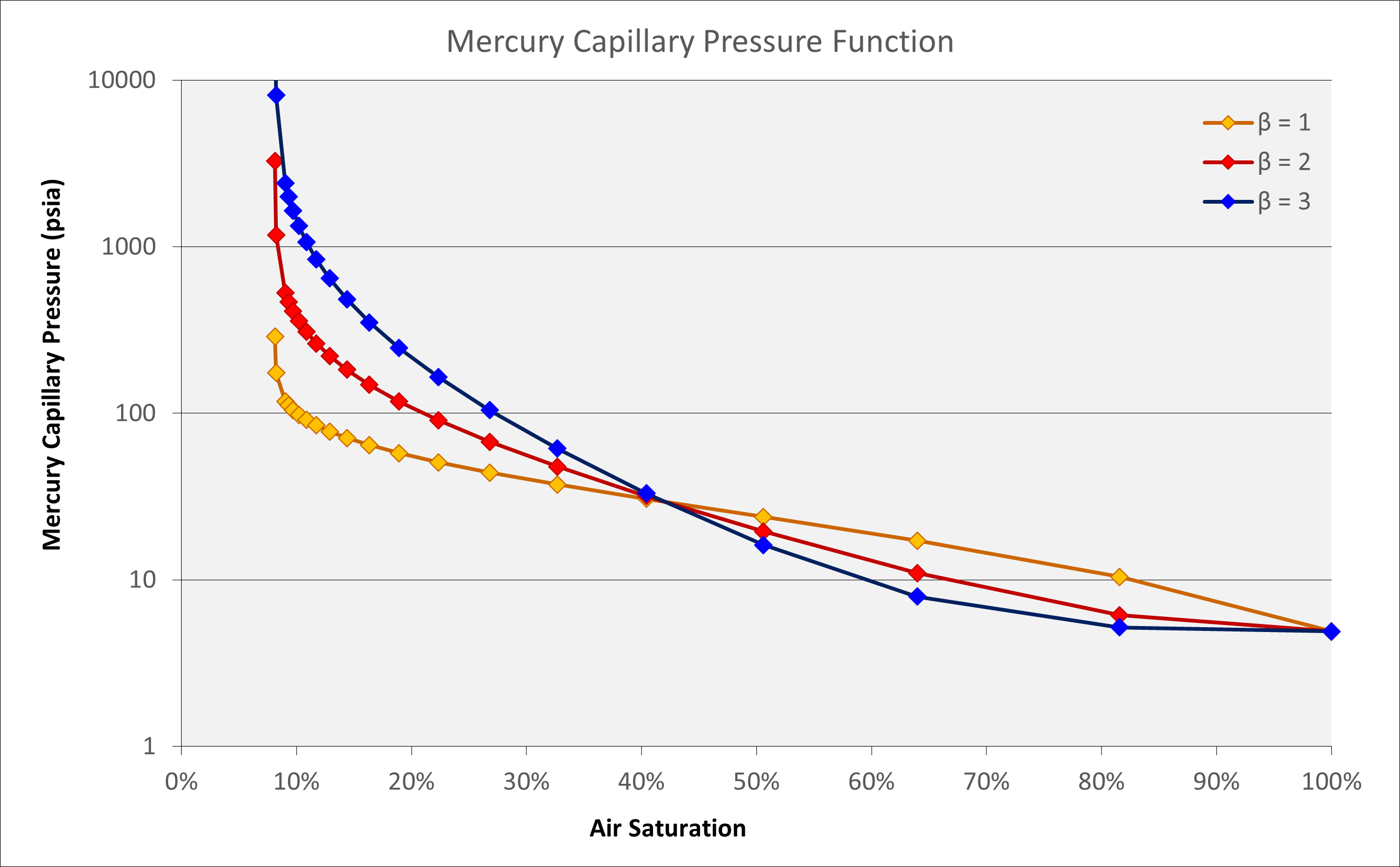
Wu determined a model for a drainage capillary pressure curve based on a form of equation originally proposed by Bentsen and Anli and implemented by Harris and Goldsmith (Harris & Goldsmith, 2001). Wu introduces a shape factor term β into the equation to modify the curvature of the P_c versus S_w curve. Combined with the displacement pressure equation above, this allows a synthetic mercury-air capillary pressure curve to be generated where σ is 485.0 dynes/cm and θ for mercury-air is 140°. In the future, this synthetic curve could be tuned to match actual rock capillary pressure measurements but otherwise, where fluids are known, the values for σ and θ can be determined using generic values or correlations. This means that the capillary pressure curve is reduced to a function of porosity and permeability and therefore it can be defined entirely using our simple rock model.

$P_{c}=P_{d}+\sigma\cdot\cos\theta\sqrt{\frac{\phi}{k}}\left(\ln{\frac{1}{S_{e}}}\right)^{\beta}$

Where:

P_c = Capillary pressure, psia
P_d = Displacement pressure, psia
σ = Interfacial tension, dynes/cm
θ = Contact angle, degrees
k = Rock permeability, millidarcy
φ = Rock porosity, fraction
Se = Effective saturation, fraction
β = Shape factor

The displacement pressure can be calculated using the empirical equation:

$\ln{P_{d}}=5.458-1.255\ln{\sqrt{\frac{k}{\phi}}}+0.081\left(\ln{\sqrt{\frac{k}{\phi}}}\right)^{2}$

The effective saturation, Se, is defined as:

$S_{e}=\frac{S_{w}-S_{wirr}}{1-S_{wirr}}$

Wu tested the shape factor β using more than 200 samples and found that this varied in the range of one to three. The factor was found to depend on lithology, pore geometry and connection. It was noted that a default value of 2 worked well for a wide range of lithology and permeability. Wu also provided guidelines for choice of the β factor:

Lithology	Pore Type	Permeability	β
Clear sandstone Carbonate	Inter-granular or inter-crystalline pores	100s ~ 1,000s mD	3
Sandstone Shaly sandstone	Micro-pores, dissolution pores	1 ~ 100s mD	2
Shale Tight sandstone	Micro-pores	<1 mD	1

For simplicity we will define the shape factor based on the modelled permeability for the specific rock type at a porosity of 20%. The relationship used is a linear transform between log₁₀(k) and β such that β = 3 at k ≥ 10,000 mD and β = 1 at k ≤ 0.01 mD.

$\beta=0.3333\log_{10}\left(k_{20}\right)+1.6667$

Where:

k₂₀ = Absolute permeability at 20% porosity, millidarcy

Use of these equations allows a synthetic capillary pressure function to be generated. For a given porosity and permeability, the mercury-air capillary pressure curve can be generated using the Wu equation.

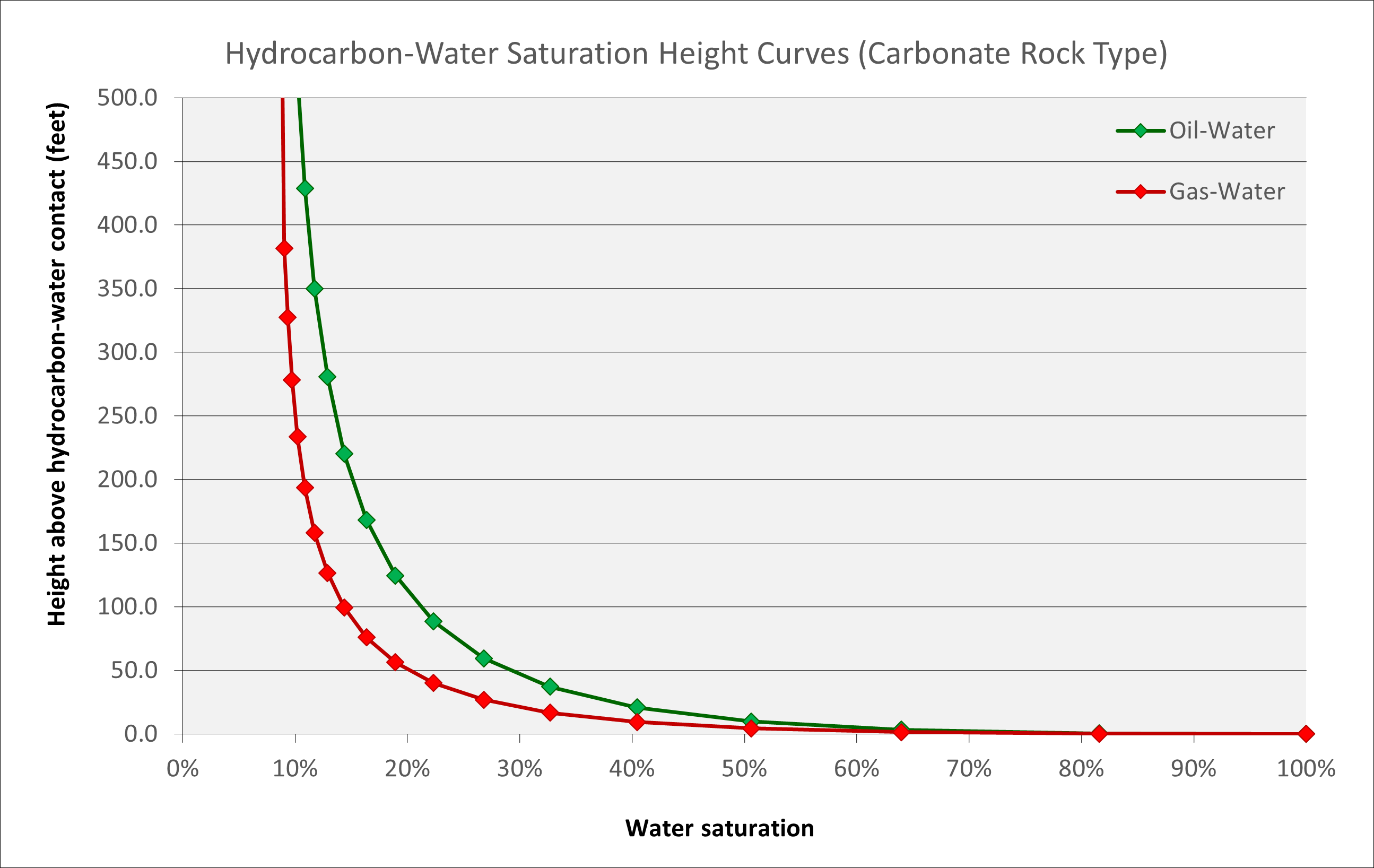
**Figure 1: Modelled capillary pressure function and variation with shape factor.**

To extend to hydrocarbon-water fluids we must determine the interfacial tensions and densities for these fluids. This allows a saturation height function for oil-water and gas-water (or gas-oil) systems to be calculated.

The water-oil interfacial tension (IFT) σ is determined using the Firoozabadi and Ramey (1988) correlation:

$\sigma_{ow}=\left[2.6628\left(\rho_{w}-\rho_{o}\right)^{-0.9136}\times\left(\rho_{w}-\rho_{o}\right)\right]^{4}$

The water-gas interfacial tension (IFT) σ is determined using the Sutton (2009) correlation modified from Firoozabadi and Ramey (1988) correlation:

$\sigma_{gw}=\left[\frac{1.58\left(\rho_{w}-\rho_{g}\right)+1.76}{{T_{r}}^{0.3125}}\right]^4$

Densities ρ_w, ρ_o and ρ_g are in units g/cm³. Reduced temperature T_r is determined from T / T_pc where the pseudo-critical temperature in degrees Rankine is calculated using an equation of State or the method of Sutton:

$T_{pc}=169.2+349.5\gamma_{g}-74.0{\gamma_{g}}^2$

For example, for a field with reservoir temperature of 244.8 degrees Fahrenheit, gas specific gravity γ_g of 0.944, density of formation water of 1.013 g/cm³ and gas density gradient of approximately 0.125 psi/ft, the gas-water IFT is 39.2 dynes/cm.

Drainage Saturation Height Function

The drainage saturation height function is applicable where the wetting phase (water) originally fills the rock pore space and is being displaced by the non-wetting phase (gas). In other words, the original water phase is being drained from the pore space.

To obtain a saturation height function from the capillary pressure in psia we can relate a given height above the gas-water contact (HAGWC) to the capillary pressure by adjusting for displacement pressure:

$P_{c'}=P_{c}-P_{d}$

$P_{c'}=\left(\rho_{w}-\rho_{h}\right)\times{HAGWC}$

Where:

ρ_w = Water density, psi/ft (0.43353 psi/ft for pure water)
ρ_h = Hydrocarbon fluid density, psi/ft
HAGWC = Height above the gas-water contact, feet

The saturation height functions for a 20% porosity carbonate (with a defined porosity-permeability transform) are shown below for oil-water and gas-water systems, assuming a factor β of 2.5.

**Figure 2: Saturation height function showing decrease in water saturation versus height for oil-water and gas-water systems.**

To generate a saturation height function we re-arrange the equations using the familiar form of the Leverett J-Function. This creates an equation that describes the water saturation for a given porosity and height above the gas-water contact.

We define the Leverett J-Function as:

$J\left(S_{w}\right)=\frac{0.216601\cdot{P_{c'}}}{\sigma\cdot{\cos\theta}}\sqrt{\frac{k}{\phi}}$

Where:

P_c = Capillary pressure above apparent gas-water contact (adjusted for displacement pressure), psia
k = Rock permeability, millidarcy
φ = Rock porosity, fraction
σ = Interfacial tension, dynes/cm
θ = Contact angle, degrees

The constant 0.216601 = (1 / 4.61678) is a result of the units chosen in the equation such that J is a dimensionless quantity. If we convert our values in psia, mD and dyne to consistent units e.g. length (L) in cm and mass (M) in lbf, we can derive a dimensionless J-Function. We note that 1 mD = 9.869233E-12 cm², 1 psia = 0.155 lbf/cm² and 1 dyne = 2.248089E-06 lbf. Therefore we need to multiply by (0.155 / 2.2481E-06) * SQRT(9.8692E-12) = 0.216601 to obtain a dimensionless J-Function.

The interfacial tension can be calculated using the Firoozabadi and Ramey (1988) correlation for oil-water or Sutton (2009) for gas-water. Sigma is typically 15 to 35 for oil-water IFT and 35 to 70 for gas-water IFT. We assume a contact angle θ for gas-water of 0° or 30° for oil-water. It does not matter whether we are considering a water-wet (θ = 30°) or oil-wet (θ = 150°) system, as the values of cos(θ) will be identical. The equation to determine water saturation can be derived from a re-arrangement of the Wu capillary pressure function expressed in S_w and substituting for J(S_w) as follows:

$S_{w}=\frac{\left(1-S_{wirr}\right)}{e^{J^{\frac{1}{\beta}}}}+S_{wirr}$

The irreducible water satuation Swirr can be estimated using the Holmes-Buckles relationship where Porosity^Q × Irreducible Water Saturation = Constant. Thus, the saturation height function is defined as:

$S_{w}=\frac{\left(1-\frac{C}{\phi^Q}\right)}{e^{J^{\frac{1}{\beta}}}}+\frac{C}{\phi^Q}$

The equation allows a drainage saturation height function to be generated for any rock type using input of five parameters: (1) porosity, (2) permeability which can be derived from porosity using a porosity-permeability transform, (3) shape factor β as either a constant or varies depending on permeability k, (4) Buckles constant C from either log measurement or rock-type / facies basis and (5) Holmes-Buckles exponent Q from either log measurement or rock-type / facies basis.

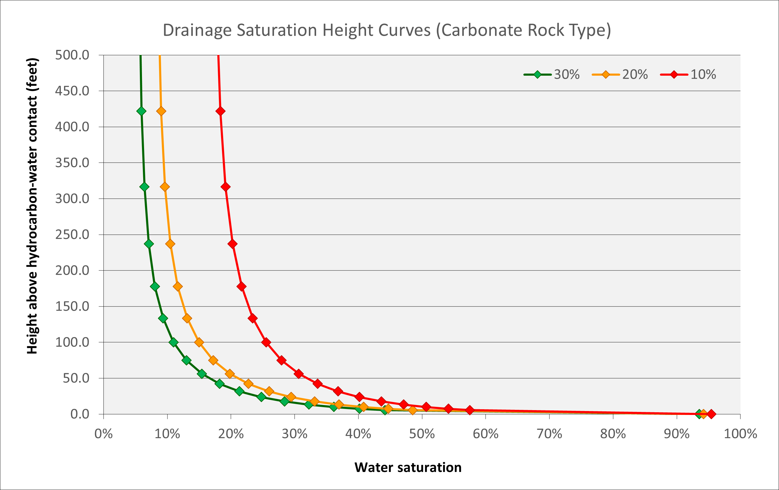
**Figure 3: Saturation height function for gas-water system in high permeability carbonate showing influence of porosity.**

Generally, this means that knowledge of porosity and the rock type alone is sufficient to generate a physically consistent and credible saturation height function. Because the saturations generated using this approach are based on underlying capillary pressures, using these predicted saturations in a static model should produce an initial reservoir condition that is in equilibrium.

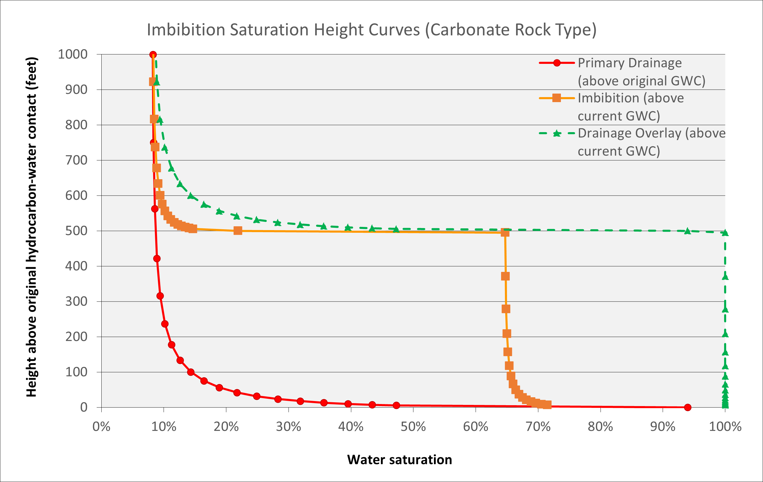
Imbibition Saturation Height Function

The opposite of drainage is referred to as imbibition. In this scenario the reservoir takes in, or ‘imbibes’, water which returns into the pore space. The saturation height function that is associated with an imbibition capillary pressure curve is different to that of a drainage capillary pressure curve.

One such scenario under which an imbibition curve might apply is associated with a deeper historical gas-water contact. This deeper contact would be associated with a drainage-type saturation height function. As the gas-water contact rises, either through gas leaking through a top-seal, or deeper burial of the reservoir which compresses the gas, the saturation height function above the current gas-water contact will become dependent on the history of the gas-water contact. The situation is not uncommon, and there are many reservoirs where the transition zone for a drainage-type saturation height function is longer than that observed on wireline logs. A specific indicator where this might be the case is where there are residual hydrocarbons evident below the interpreted free water level.

An illustration of the phenomenon is shown below. This shows a carbonate reservoir with uniform 20% porosity where the original or paleo gas-water contact (associated with the drainage water saturation profile shown in red) has risen by 500 feet. The current gas column is therefore located a a depth between 500 to 1,000 feet above the original gas-water contact. The application of an equivalent drainage saturation height function at the new depth would yield a saturation profile shown by the green dashed line. However, the imbibition behaviour whereby water is being drawn back into the formation as the contact rises and the capillary pressure is thus reduced, affects the gas saturation in the swept zone below the current gas-water contact and in the reservoir above it. Below the new contact the water encroachment displaces most of the gas, but there will be residual gas that cannot be displaced. The residual gas saturation is a function of the initial gas saturation and porosity. Above the new contact the reduction in capillary pressure leads to an increase in water saturation, but the overall water saturation is lower than it would be under a pure drainage situation. The result is that there is a shorter transition zone for the imbibition saturation height function than suggested by the drainage saturation height function.

It is observed that the water saturation above the gas-water contact under an imbibition capillary pressure is lower than that under a drainage capillary pressure. Therefore, water saturations determined using a drainage saturation height function would underestimate the hydrocarbons in place.

**Figure 4: Imbibition saturation curve arising from rise in contact to current location from deeper paleo contact depth.**

An empirical method to implement the imbibition saturation height function is described by Adams (2003). This is the “imbibition from drainage” method which is based on fitting a curve to the difference between drainage and imbibition measurements from laboratory data. The slope ‘s’ and intercept ‘int’ of the difference in water saturation is determined as follows:

$S_{wI}=S_{wD}-\Delta{S_{w}}$

$\Delta{S_{w}}=s\cdot{S_{wD}}+int$

$int=a+b\cdot{\ln{k}}+c\cdot{S_{wD,orig}}$

Where:

S_wI = Imbibition water saturation for current gas-water contact, fraction
S_wD = Drainage water saturation for current gas-water contact, fraction
k = Rock permeability, millidarcy
S_wD,orig = Original drainage water saturation at current depth prior to imbibition, fraction
S_wD,min = Minimum drainage water saturation at crest prior to imbibition, fraction

Adams’ approach suggests that laboratory data are used to optimise the unknown variables. Using the published laboratory datapoints an approximation can be made. The slope is effectively constant and weakly correlated against the minimum water saturation and the permeability. Therefore, an average of the two regressions plotted by Adams is used to determine the slope s. To determine the co-efficients, a, b and c we note that at the crest of the reservoir the imbibition and drainage curves should match e.g., S_wI = S_wD. Therefore, we can re-arrange the equations to derive the following:

$s=\frac{\left(0.0942\cdot{S_{wD,min}}+0.8323\right)+\left(-0.0077\cdot{\ln{k}}+0.9039\right)}{2}$