Modelling of fluid properties is commonly referred to as ‘PVT’ which stands for Pressure, Volume and Temperature and reflects the observed phenomenon that changing any one of these three properties will result in consequential changes to the other two. The prediction of these properties is achieved via a model, which takes fluid measurements and desired conditions (such as temperature and pressure) as its inputs and provides the PVT and other properties as its outputs. A challenge is that whilst more advanced models exist, these usually require a description of the fluid which breaks it down into a compositional description of its components. This can be obtained via laboratory analysis. If the laboratory analysis has not been performed, the analysis options are more limited. Presented here is a method that allows a good approximation of the fluid composition to be obtained from field separator measurements alone.
Predicting fluid properties using an equation of state (EoS) model is a routine task these days. If we can model our fluid with reasonable accuracy, we can produce the necessary inputs to describe that fluid for a reservoir simulator. These properties include the variation of fluid volume and viscosity as temperature and pressure are varied. The accuracy of the modelled fluid properties will affect the reservoir simulator’s predictions of production rates and overall recovery factor of the hydrocarbons initially-in-place.
The inputs used for these fluid models vary. The simplest input data is referred to as field data, and are measurements taken of the oil and gas produced from the wells following the initial separation process. This data is easy to obtain and is always available. The most complex data is a compositional breakdown that uses a combination of gas chromatography and mass spectrometry to analyse a fluid and provide a detailed breakdown of its constituent components. This reasonably easy to obtain for the gas component, and is commonly performed in the field during well test operations, but for a reliable analysis the current practice is to collect representative samples and send those to a laboratory for analysis.
The results from the laboratory analysis are a detailed breakdown of the hydrocarbon mixture. The equipment used actually measures the fractions of each component according to its percentage weight of the overall mixture, and using known (or estimated) molecular mass for each component, this is converted into a mol percentage (mol%). That is to say, for any given number of molecules in a mixture, what percentage of them comprise a particular compound. The mol% breakdown can then be used with EoS models to predict the mixture’s fluid properties.
The option to use more advanced EoS models is not an option where only field data is available. Historically the oil industry has developed and published several correlations to predict fluid properties in the absence of laboratory tests. Predictions using EoS would be possible if it were possible to estimate the composition from field measurements alone. If an analogue fluid exists, then that composition could be used instead, although this approach requires a large database of fluid compositions and could not be considered a generalised approach. The problem is that there are often just three (or six if non-hydrocarbon impurities are included) field measurements available but 11 (or 14) unknowns to predict. A successful approach to estimate composition from field data for gas-condensates and volatile oils using non-linear regression has been published (Spivey and McCain, 2013). No generalised estimation approach for any hydrocarbon fluid, including dry gas and black oil, exists (at least to the best of my knowledge – apologies if there is one that I’m not aware of).
Building on insights from Spivey and McCain, a new genetic algorithm was developed to estimate composition from field data that can be applied to any type of hydrocarbon. This generalised algorithm predicts a non-unique composition that matches the target field data. By running a Monte Carlo simulation, it is possible to also quantify the uncertainty in the composition of each component, and choose the mean values as representative of the ‘best’ composition that matches the available field data.
Current Approaches to Predicting Fluid Properties
Approach 1: Use of Correlations Based on Empirical Data
When oil and gas is produced to the surface, the first process that the fluid encounters is typically a separator. This vessel contains the fluid at a controlled temperature and pressure that is significantly lower than the reservoir pressure that it originally existed at, but is also above atmospheric pressure and temperature. In the separator, dissolved gas in oil will bubble out of solution (much like opening a bottle of soft drink allows the bubbles of carbon dioxide to escape) and vaporised oil will condense to form liquid (similar to how dew forms on the ground when overnight temperatures fall allowing moisture in the air to condense). The process results in three easily measured properties:
- The relative density of oil (usually measured relative to water = 1 or using API gravity)
- The relative density of gas (usually measured relative to air = 1)
- The producing ratio of gas to oil measured in scf/stb in customary field units
In addition, measurements for the compositional fraction of non-hydrocarbon impurities are sometimes taken. These impurities are carbon dioxide, nitrogen and hydrogen sulphide.
Using these three to six input variables, and optionally taking into consideration the separator temperature and pressure conditions, perhaps over a hundred different correlations (I’m guessing but there are many) for various PVT properties have been published. The correlations are undoubtedly useful, and allow PVT properties to be obtained in the absence of laboratory analysis.
However, they all suffer from several disadvantages. These include:
- Datasets are used for each correlation and application of the equation to fluids whos properties fall outside the bounds of the input dataset leads to extrapolation and potential inaccuracy.
- The datasets used tend to have geographical bias. Whilst it has been shown that a similar hydrocarbons from two different geographical regions will have similar properties (e.g., a fluid with exactly the same composition will have exactly the same properties irrespective of the region in which it occurs), each geographical region tends to have a narrow range of different hydrocarbons. Thus application to a different region may not be applicable.
- A different correlation is needed for each PVT property, meaning a complete set of fluid properties may be made up of correlations based on different datasets, and are thus unlikely to be consistent.
- There is inconsistency in how the input parameters are defined and used. For example some correlations require gas-oil ratio at the separator, and others require total gas-oil ratio which includes the rarely measured stock tank gas volumes which are vented or flared.
- Flash calculations to predict oil and gas ratios at different conditions are impossible, so more advanced techniques such as production of phase envelopes and use of process simulation software also also not possible.
Approach 2: Application of an EoS to a Known Fluid Mixture Composition
For pure fluids, such as methane or carbon dioxide, a great deal a research effort has been invested into studying and modelling the behaviour of these pure compounds. One such open source library is the CoolProp library. This wonderful library is released with several wrappers for different languages, including Java, which means it can be incorporated into many different applications. Specifically in relation to Java I can confirm that it compiles and runs on Windows, Linux and MacOS as I contributed a patch that fixed an issue with their MacOS flavoured wrapper. Within the Pyrus suite of oil and gas tools, the PVT modelling tool uses CoolProp for the underlying EoS.
As petroleum engineers we very rarely deal with pure fluids. Even if we are looking at something like carbon dioxide sequestration, we are likely to be dealing with a mixture of mostly pure carbon dioxide, plus a smaller fraction of contaminants such as nitrogen or air etc. With hydrocarbon fluids, there are literally hundreds of thousands of possible compounds that can be found in any oil or gas, although the gases (thankfully) tend to have a large number of simple compounds such as methane, ethane, propane etc. These multiple heavier components can be grouped into one or more pseudo-components that reflect the paraffinic, napthenic and aromatic predominance. Characterisation of this plus fraction component is a detailed separate discussion. Suffice to say, it has a large influence on the fluid property predictions when applying an EoS to a composition. With this in mind, laboratories now provide breakdowns for pseudo-components with single carbon numbers up to C36+ or higher, rather than just a C7+ fraction.
With a detailed fluid composition, a cubic EoS can be used. These equations have a long history, tracing their roots back to Nobel prize winner van der Waals in 1873. In over a century and a half many variations to the original cubic EoS have been investigated and published, and although they are not able to perfectly predict all fluid properties, they have stood the test of time and are commonly utilised today. Essentially, the world is still waiting for someone to invent or discover a better approach.
The Pyrus suite incorporates an implementation of a cubic EoS. This imposes a simpler user interface onto the problem, and allows more advanced fluid properties to be determined. The challenge is that is necessary to have a detailed fluid composition to use this approach, and if only field data are available, then usually the conclusion is that a cubic EoS cannot be used.
The New Algorithm: Bridging the Gap
Given a problem of determining many unknowns from far fewer knowns, the brute force solution is essentially a trial and error search methodology. The strategy is to first guess what the unknowns are; in our case a fluid composition. Using the composition, a cubic EoS is applied to predict the field data. The predicted properties are then compared against the known measured properties. If the properties match, then excellent, you’ve found the correct composition. If they don’t match, then you can use the answer obtained to come up with a better match. Simply rinse and repeat the cycle until you converge on a solution that is close to matching.
I mean, how hard could it be? Well the answer to that question can be computed mathematically as how many different combinations are there. We have 14 unknowns, and for each of these let’s say there are just 101 different options e.g. 0%, 1%, 2% etc. up to 100%. Then the number of possible combinations is a staggering 3.13 × 10¹⁷. Such a number is hard to comprehend. To put it into context, we can do a similar calculation for picking winning lottery numbers. For example the chance of correctly picking 6 numbers from a pool of 1 to 47 choices, is 1 in 10,737,573 or roughly 1 in 11 million. This means that you are approximately 30 billion times more likely to win the lottery than pick the correct composition. And this is just for a composition where each component’s fraction is expressed in integer percentages. In reality we need to define these with several decimal places, at which point the number of combinations becomes staggeringly incomprehensible. In short, this is a massive search space.
The problem is by no means unique, and solutions to these types of problems have given rise to a family of various non-linear regressions such as the Levenberg–Marquardt algorithm. These algorithms minimise the error between the desired solution and the current solution by mathematically converging towards an optimal solution. This is the approach used by Spivey and McCain.
Personally, I’ve always been a fan of genetic algorithms. These adopt a different approach to achieving convergence, and take inspiration from nature to evolve a better solution as measured by a fitness function. Fundamentally they are doing the same thing as a non-linear regression: searching for a good (but not necessarily the absolute best) solution from a massive set of possible solutions. Where they differ is in their underlying mechanics. Where non-linear regression is mathematically robust, a genetic algorithm is more of an engineering approach that favours obtaining better solutions even though it may not be clear exactly how the solution was found. Being an engineer, as opposed to a mathemetician, the new algorithm was developed principally to satisfy curiosity: would it work to find a composition that matches field data?
Designing the Genetic Algorithm and Its Fitness Function
In the genetic algorithm a population of candidate compositions, called a MixtureOrganism in my code, is artificially generated. Each MixtureOrganism is defined by a random array of genes from which the composition can be obtained. The fitness of each MixtureOrganism is evaluated based on how well its composition matches the target field data, and the fitness of each MixtureOrganism in the population is ranked. Based on the rankings, pairs of candidates are chosen at random (with preference to fitter MixtureOrganisms – Darwin’s “survival of the fittest” being very much applied here). Every two parent candidates ‘breed’ by swapping their genes. Genes from both parent A and parent B end up in the child. There is a chance that some genes are randomly mutated, which introduces variety into the population. Enough children are bred from the existing population until their are a sufficient number of children to form a new generation population. This process is repeated until the fitness of the best MixtureOrganism is high enough that the predicted field measurements obtained from an EoS applied to the composition are essentially the same as the measured field data.
The genes are represented by our 14 unknowns where xn is a value for that gene:
| CO2 | N2 | H2S | CH4 | C2H6 | C3H8 | IC4 | NC4 | IC5 | NC5 | C6 | C7+ | C+MW | C+GAMMA |
|---|---|---|---|---|---|---|---|---|---|---|---|---|---|
| x1 | x2 | x3 | x4 | x5 | x6 | x7 | x8 | x9 | x10 | x11 | x12 | x13 | x14 |
The fitness function itself is related to a mathematical least squares error approach, but has some little tricks that I discovered really helped to improve the convergence. I won’t reveal them here for two reasons: (1) they would involve a lot of laborious explanation and (2) I might choose to publish the findings in the future.
In comparison to the a non-linear regression, the key difference here is that rather than mathematically trying to converge to a better solution, better solutions emerge through their superior genes preferentially remaining in the population.
This gives rise to a key advantage of the genetic algorithm approach: the algorithm has no knowledge of how to find a fitter solution. It can only distinguish between a ‘more fit’ or ‘less fit’ candidate. This means that it can be used to evolve MixtureOrganisms that match fluid in the whole spectrum of dry gas, wet gas, gas-condensate, volatile oil or black oil. Once the best (fittest) MixtureOrganism is identified, we obtain a composition from its genes, and can then determine any fluid properties we like using an EoS approach instead of correlations.
Examples and Validation
Proof of Concept: Recreate Composition from Field Data Obtained Using Known Composition
To test the performance of the genetic algorithm a simple methodology was proposed:
- Simulate field data using an EoS for a known composition.
- Run the genetic algorithm on the simulated field data to recreate the composition.
- Compare the original composition to the recreated composition.
The conditions for this test are favourable, since the same EoS is used to simulate the field data as used by the genetic algorithm to generate the fitness function for each MixtureOrganism. This eliminates any differences in the EoS as a variable for testing performance of the genetic algorithm.
A set of compositions representing a broad spectrum of different hydrocarbons was used to test the proof of concept, supplemented by fluid from the Pasca A gas-condensate field in Papua New Guinea. The compositions are obtained from Table 1.2, Characterization and Properties of Petroleum Fractions, M. R. Riazi (2005).
| Component | Dry Gas | Wet Gas | Gas Condensate | Volatile Oil | Black Oil |
|---|---|---|---|---|---|
| CO2 | 0.0370 | 0.0 | 0.0018 | 0.0119 | 0.0209 |
| N2 | 0.0030 | 0.0 | 0.013 | 0.0051 | 0.0009 |
| H2S | 0.0 | 0.0 | 0.0 | 0.0 | 0.0189 |
| CH4 | 0.9600 | 0.8228 | 0.6192 | 0.4521 | 0.2918 |
| C2H6 | 0.0 | 0.0952 | 0.1408 | 0.0709 | 0.1360 |
| C3H8 | 0.0 | 0.0464 | 0.0835 | 0.0461 | 0.0920 |
| IC4 | 0.0 | 0.0064 | 0.0097 | 0.0169 | 0.0095 |
| NC4 | 0.0 | 0.0096 | 0.0341 | 0.0281 | 0.0430 |
| IC5 | 0.0 | 0.0035 | 0.0084 | 0.0155 | 0.0138 |
| NC5 | 0.0 | 0.0029 | 0.0148 | 0.0201 | 0.0260 |
| C6 | 0.0 | 0.0029 | 0.0179 | 0.0442 | 0.0432 |
| C7+ | 0.0 | 0.0101 | 0.0685 | 0.2891 | 0.3040 |
| C+MW | - | 113.0 | 143.0 | 190.0 | 209.8 |
| C+GAMMA | - | 0.794 | 0.795 | 0.8142 | 0.844 |
Field data were simulated using the EOS by passing the reservoir fluid through a two-stage separation process (high pressure separator @ 800 psia and 150.0 °F followed by a low pressure separator @ 150 psia and 50.0 °F). The simulated field data for each of these fluids that was used as an input to the genetic algorithm is shown in the table below:
| Field Data | Dry Gas | Wet Gas | Gas Condensate | Volatile Oil | Black Oil |
|---|---|---|---|---|---|
| Oil API Gravity | 310.3 | 55.3 | 55.7 | 49.7 | 47.6 |
| Gas Relative Density (air = 1) | 0.591 | 0.705 | 0.772 | 0.853 | 0.959 |
| Gas-Oil Ratio (scf/stb) | ∞ | 170,545 | 8,470 | 1,019 | 1,046 |
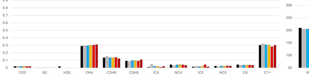
The genetic algorithm was able to generate compositions for all of these fluids, demonstrating its applicability to a wide range of fluid types. Because the solutions are non-unique, a Monte Carlo approach was adopted, with 100 different compositions predicted per fluid type. The range of each component, as well as the mean value are compared to the initial reference composition. The statistical cases shown are defined as P{X}, where P{X} is the composition for which X% of CH4 fractions are smaller that its value. In general, towards the P1 end of the range we have lighter compositions and towards the P99 end of the range we have heavier compositions. However, this is not a strict rule. In addition, the phase envelope for each composition was generated using the Peng-Robinson cubic EoS and compared against the range of predicted compositions.
Note that in these charts the solid black represents the original reference composition, and amber is the mean composition as determined by taking the mean result predicted for each component during the Monte Carlo run.
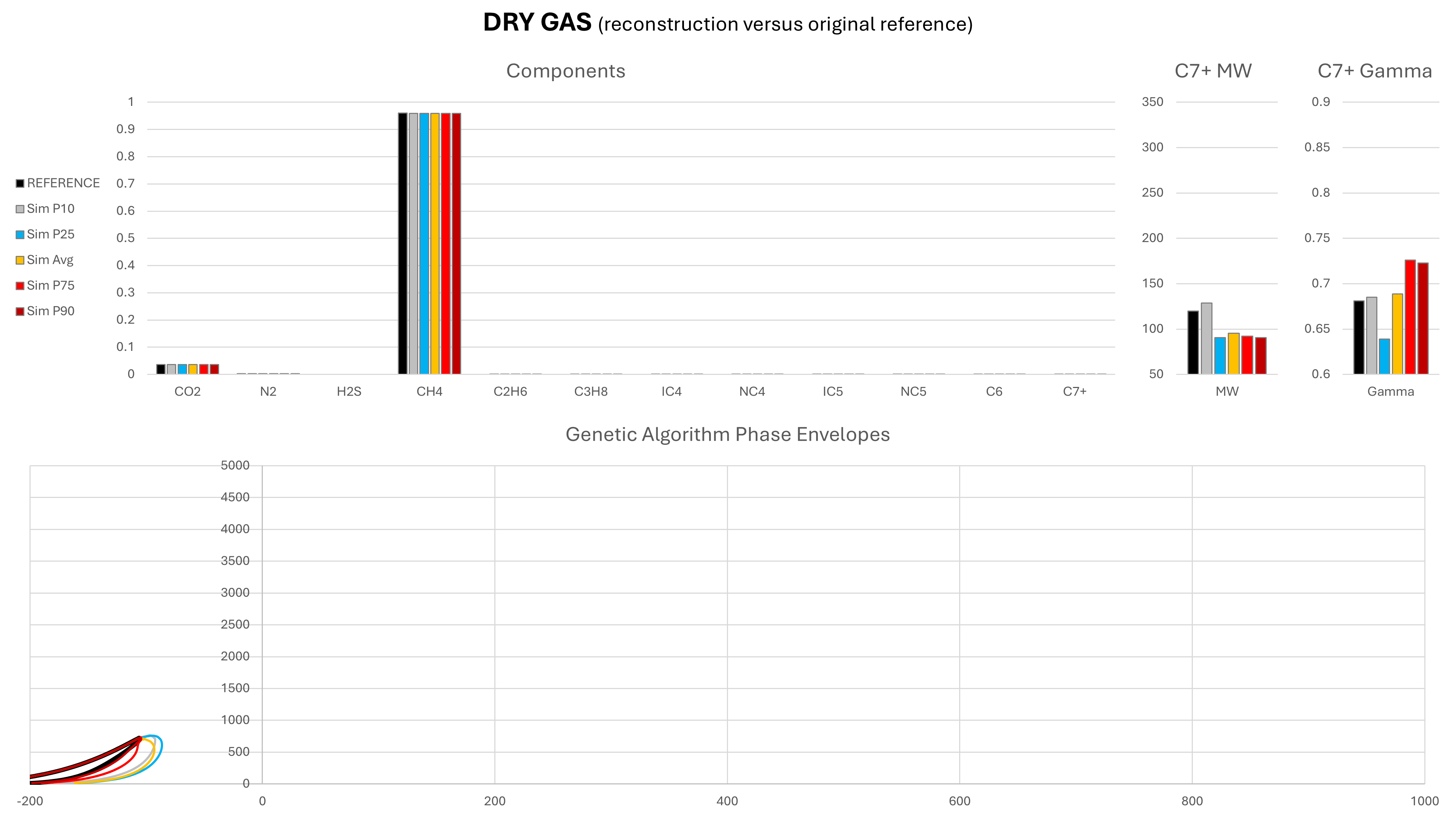
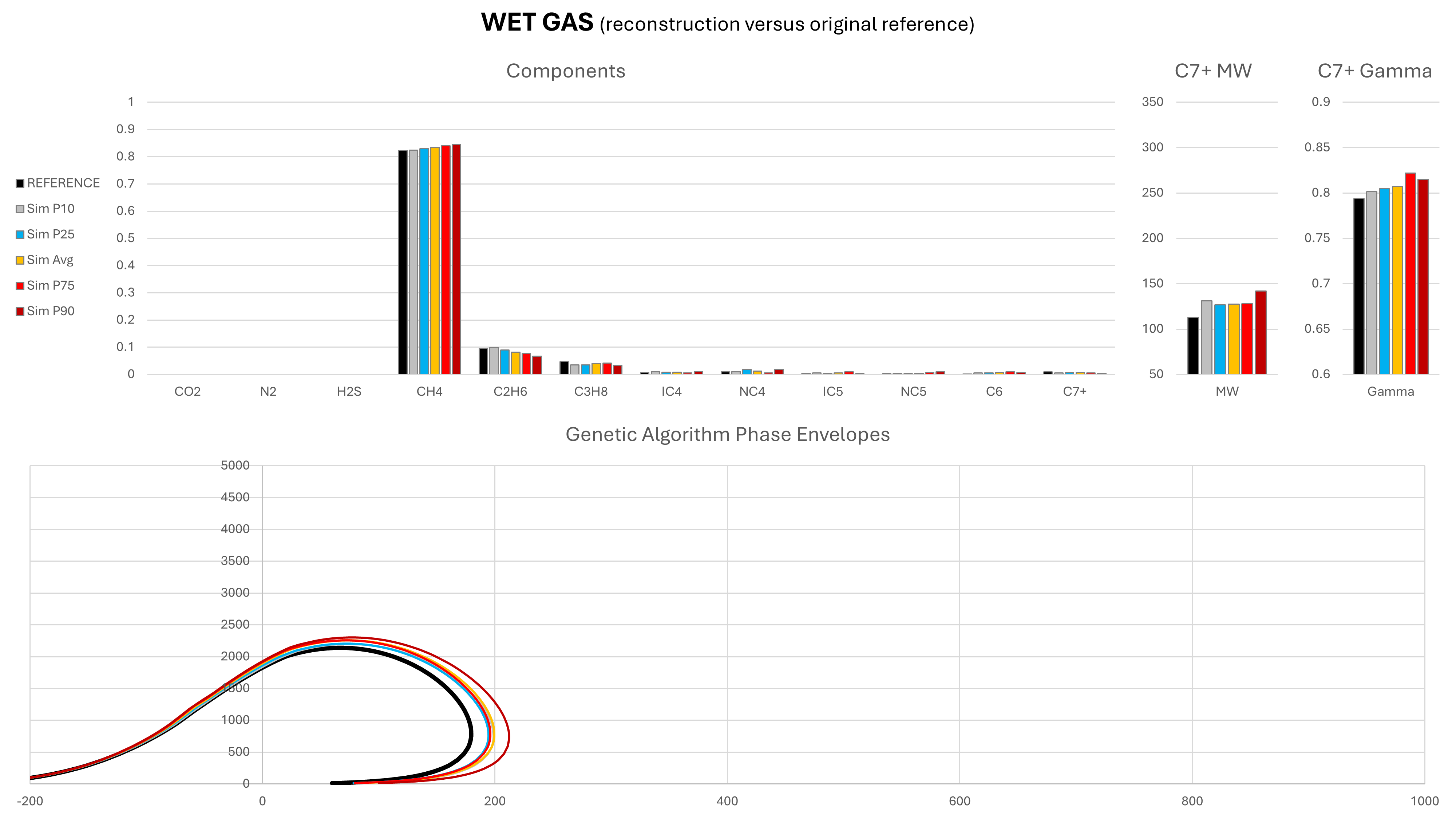
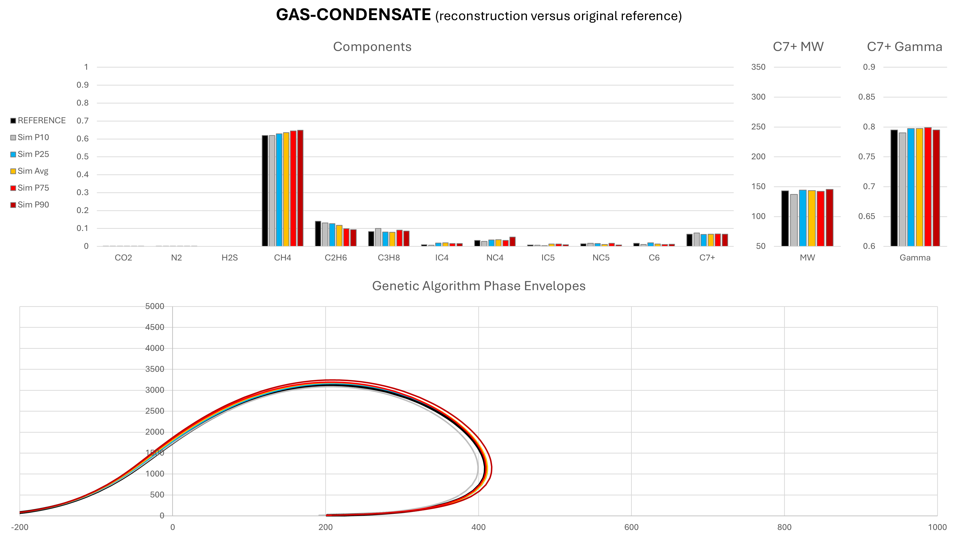
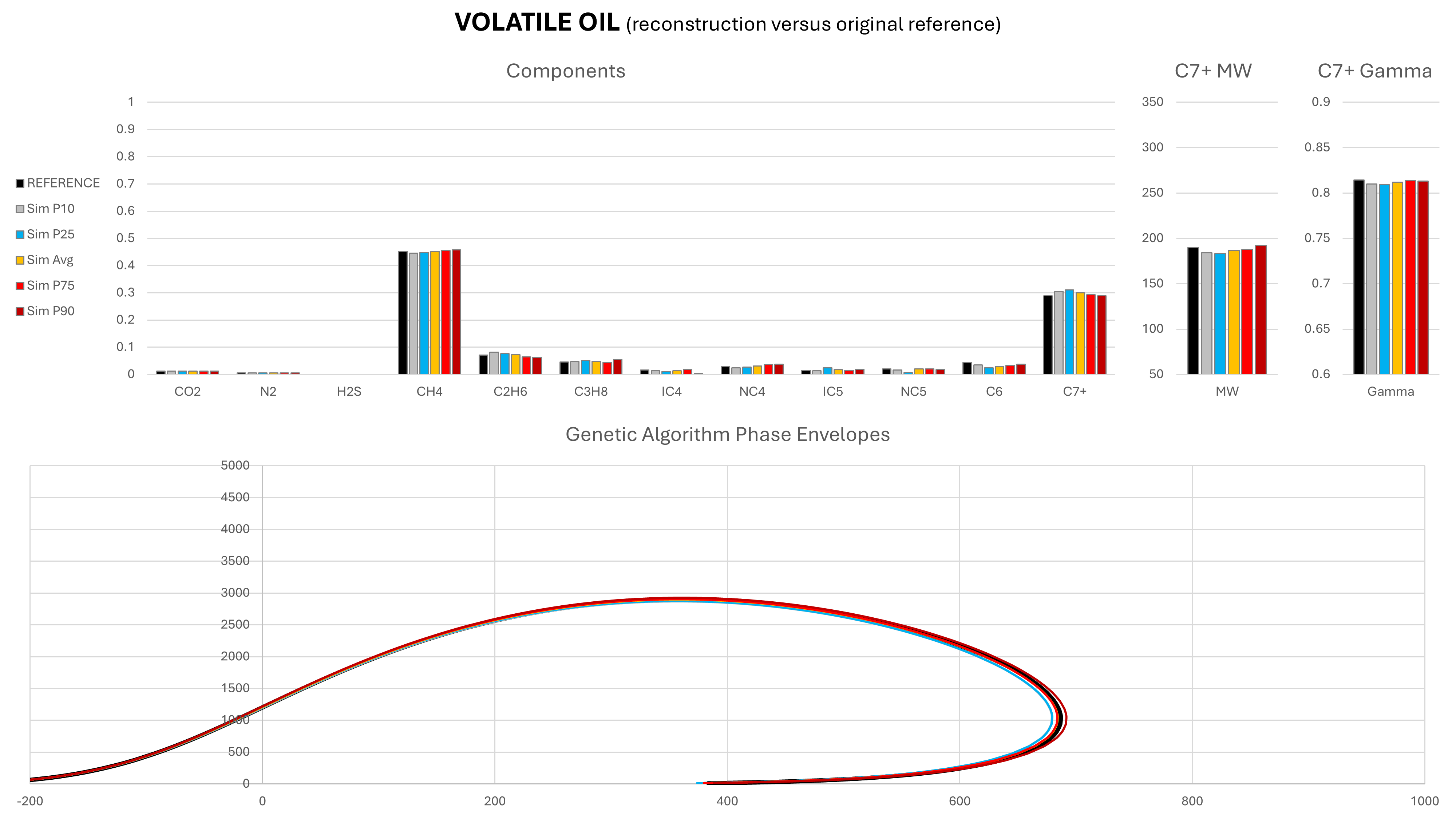
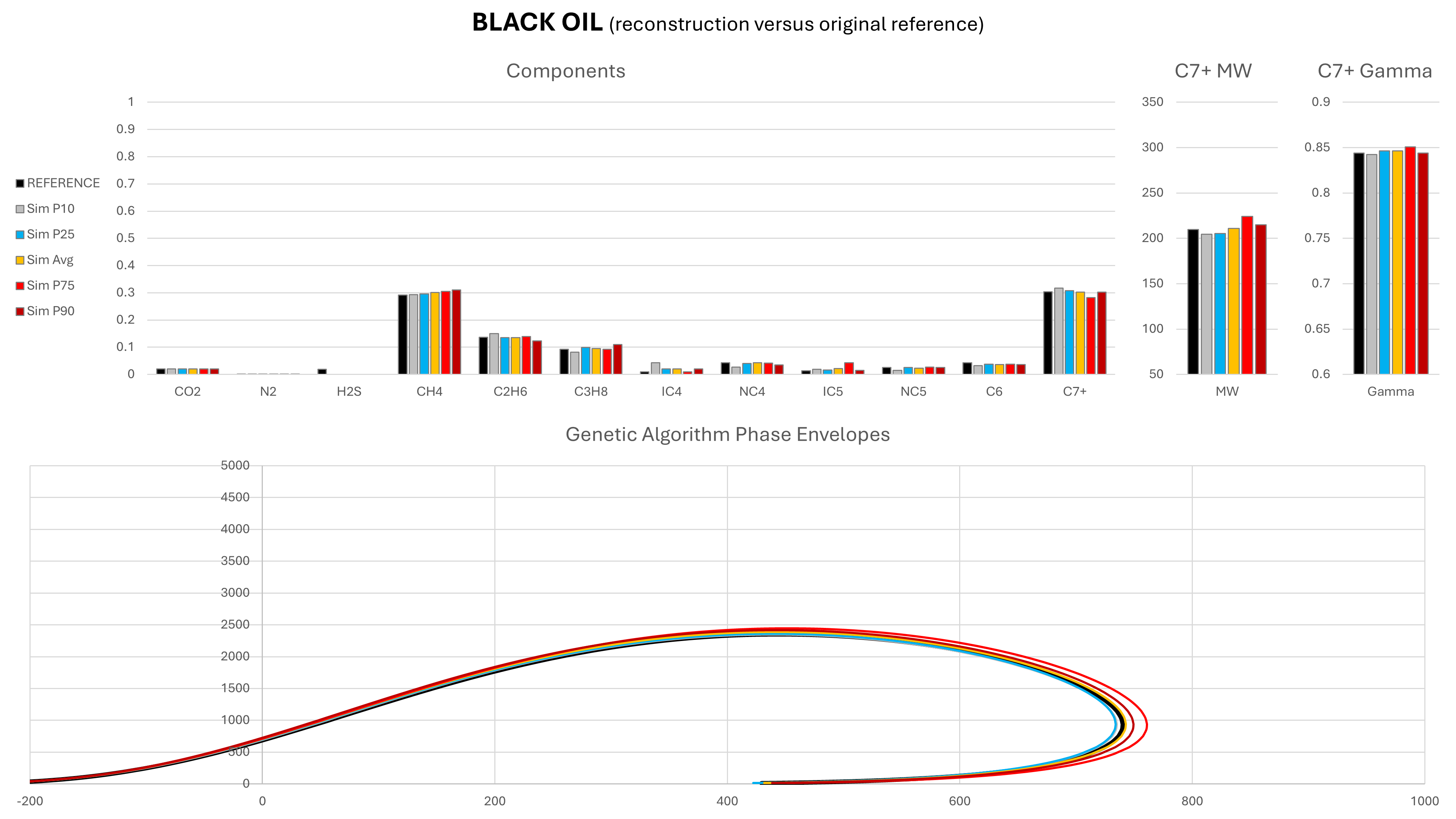
It can be seen that in most cases, the predicted mean composition is a very close match to the actual reference composition. Most compositional components are very similar to the original reference composition from which the simulated field data were derived. It is the C7+ molecular weight and relative density that exhibits the greatest variability, particularly for the dry gas and wet gas. It is this variability that drives the differences in the phase envelopes. Despite the variability, the saturation envelopes are comparable, which suggests that the GA-derived composition could potentially be used to predict dewpoint or bubblepoint pressures in a similar manner to existing correlations.
Comparison Against Correlations for Predicting Fluid Properties
The real test is to check the method stacks up against other published data as an alternative for application of correlations to field data. If an estimated composition can be produced that is at least as good as existing correlations (or improves upon them), then this opens the door to performing consistent PVT analysis with field data alone. This is not to say that such an approach should replace obtaining a compositional breakdown from laboratory analysis. Rather it provides an alternative option should that data not be available.
Furthermore, knowledge of the composition allows PVT tables to be generated for reservoir simulation that are consistent. That is, the saturation point at reservoir temperature, the formation volume factor and viscosity are all derived from the same composition and using the same EoS (where applicable).
For our comparison we have initially used compositions from Ahmed (2006) as the source of a small set of example reservoir fluids, for which field data measurements are available.
| Field Data | Oil #1 | Oil #2 | Oil #3 | Oil #4 | Oil #5 | Oil #6 |
|---|---|---|---|---|---|---|
| Reservoir Temperature (°F) | 250 | 220 | 260 | 237 | 218 | 180 |
| Oil API Gravity | 47.1 | 40.7 | 48.6 | 40.5 | 44.2 | 27.3 |
| Gas Relative Density (air = 1) | 0.851 | 0.855 | 0.911 | 0.898 | 0.781 | 0.848 |
| Gas-Oil Ratio (scf/stb) | 751 | 768 | 693 | 968 | 943 | 807 |
A comparison of the bubble point pressure in psia obtained using several correlations versus those calculated from different EoS together with the composition obtained from the genetic algorithm is shown. The EoS used are Peng-Robinson (PR), Enhanced Predictive Peng-Robinson (EPPR78) and EPPR78 with the α value for the C7+ fraction slightly tuned by multiplying by 1.03×. The tuning applied in the last EoS is done as the C7+ pseudo-components do not fully capture the effect on the phase envelope of very heavy components. A different approach would be to split to C7+ fraction into several components before running the EOS, but tweaking the α parameter is simpler. For the purposes of testing whether the compositions obtained from the genetic algorithm is comparable to results obtained from correlations, it is a reasonable starting point. The average relative error (bias) and average absolute relative error (accuracy) are shown for these six oils.
| Metric | Measured | Al Shammasi | Lasater | Vasquez-Beggs | Velarde | Valko-McCain | GA (PR) | GA (EPPR78) | GA (EPPR78 + α 1.03×) |
|---|---|---|---|---|---|---|---|---|---|
| Pb (Oil #1) | 2,392 | 2,163 | 2,263 | 2,319 | 2,322 | 2,531 | 1,972 | 2,312 | 2,395 |
| Pb (Oil #2) | 2,635 | 2,480 | 2,595 | 2,742 | 2,644 | 2,676 | 2,082 | 2,516 | 2,615 |
| Pb (Oil #3) | 2,066 | 1,916 | 1,921 | 2,043 | 1,914 | 2,116 | 1,753 | 2,020 | 2,089 |
| Pb (Oil #4) | 2,899 | 2,966 | 3,061 | 3,469 | 3,120 | 2,969 | 2,435 | 2,984 | 3,050 |
| Pb (Oil #5) | 3,060 | 2,774 | 3,065 | 3,049 | 3,128 | 3,265 | 2,467 | 2,984 | 3,112 |
| Pb (Oil #6) | 4,254 | 3,467 | 3,435 | 4,095 | 3,444 | 3,393 | 2,748 | 3,477 | 3,635 |
| Pb ARE | - | -7.5% | -4.0% | 3.1% | -2.7% | 0.3% | -20.8% | -5.0% | -1.2% |
| Pb AARE | - | 8.5% | 6.3% | 5.2% | 6.6% | 7.0% | 20.8% | 5.3% | 3.9% |
The results show that when used with a suitable equation of state, the recreated compositions from field data provide a predictive capacity for the bubble point that is at least as good as correlations commonly applied for this purpose. Whilst the approach probably won’t be replacing the use of correlations for this purpose any time soon (a correlation is still far simpler and quicker to utilise), this does demonstrate that the approach is valid. Furthermore, if more advanced PVT analysis is required, this can be achieved using the composition created using the genetic algorithm.
Analysis and Discussion
The examples clear show that it is possible to recreate a composition from field data alone. The modelling of the separation process accurately does affect the results, but as shown by the difference in the simulated and measured field data for Pasca A, provided the field data are thermodynamically consistent for that composition, the genetic algorithm will still converge to a result that is close to the reference composition.
Although the result obtained from the genetic algorithm is non-unique, when combined with a Monte Carlo technique, the approach provides a statistical range of uncertainty around each component, and the mean composition that is predicted is a good match to the actual reference compositions used in these examples.
Where no laboratory analysis is available to obtain a compositional breakdown, the new method can be used instead. This allows techniques only possible with knowledge of the composition to be used, including creation of consistent PVT black oil tables for reservoir simulation, or even application of compositional simulation should be required.
The use of a Monte Carlo technique to arrive at multiple solutions is an inherent benefit of the method; it is able to quantify a range of uncertainty around predictions. For analysis using field data, petroleum engineers have tended to use correlations, or estimate a composition using analogue datasets or a non-linear regression technique. These methods all produce a single predicted value.
The genetic algorithm combined with a Monte Carlo approach will produce a distribution for any predicted value. Thus rather than just predicting the bubble point, it will indicate the level of confidence in that prediction. This could potentially be used to validate measurements as it could identify inconsistencies in measured data. It can also help to provide a range of compositions for process simulation which would allow uncertainty in the fluid properties to be captured in the design process. Often a representative sample is chosen for design purposes and is defined the the basis of design. However, there are several reasons why that composition might have inaccuracies: the characterisation of the heavy fractions being notable here as the paraffinic, napthenic and aromatic content might be very different to that assumed by the laboratory in producing the mol% composition from the measured wt% composition.
Although the method appears to work well, this is still very much in an early stage of development. A few areas for improvement have been identified:
- Separation modelling: The test separation process that is simulated does not closely match the actual field data measurements for Pasca A. A more nuanced approach in comparison to the simple single flash for the separator and stock tank that is used to model the separator process is possibly required. To objective would be to obtain a better match between simulated test separation parameters and actual measured parameters.
- Genetic algorithm optimisation: The current implementation of the fitness function and population selection appears to work successfully to identify matching compositions. However, whilst running the algorithm can sometimes get stuck with a poor quality population and it can take time for better quality
MixtureOrganisms to emerge via mutation. Research into different genetic algorithm strategies and their implementation, including techniques such as elitism and speciation, might reveal more optimal approaches that can accelerate discovery of a fit solution. - GPU processing: The genetic algorithm and Monte Carlo technique is an inherently parallel calculation. Calculations for the fitness function on each
MixtureOrganismin the current generation’s population can be conducted in parallel, and furthermore each genetic algorithm result in a Monte Carlo simulation can also be run in parallel. The Pyrus code has been written to take advantage of parallelisation on the CPU. This could be extended to the GPU, much like with current AI workloads where the many parallel cores in GPUs are used to train neural nets.
Conclusion
A new method to generate a compositional breakdown from field separator measurements alone has been devised. The method is based on a genetic algorithm combined with a Monte Carlo approach, to estimate a best fit composition to the field data, in addition to a range of possible compositions.
It is demonstrated that where an initial composition is provided, simulated field data obtained from that composition can be used to recreate the original composition. Actual field measurements do not match those obtained from the currently simulated separation process. Nonetheless, the algorithm is able to generate a composition that is close to the known composition. This suggests that improvements to the modelling of the separation process that is part of the algorithm would lead to improved accuracy.
The benefits of the approach are that it allows a greater range of PVT fluid characterisation to be performed in comparison to the limited approaches available from the use of correlations alone. In particular, it allows process simulation of produced fluids to be undertaken in the absence of a laboratory analysis to provide the composition.
The accuracy of the fluid property predictions using the estimated composition are at least as good as those obtained from the best performing correlations.
Where to Next?
An enigma presents itself with this new method.
Whilst I’ve had the idea of doing this for many years, I’ve never had a need to try it out, so it has sat patiently on a shelf in my mind. Whilst writing the GUI for saturation height function modelling in Pyrus, I briefly had a thought that I would need to be able to create compositions from input of field data alone. This was the impetus to start implementing and testing whether a genetic algorithm would work. Surprisingly it only took a couple of weeks to create a working algorithm, and perhaps more surprisingly, in those two weeks I discovered a workaround that meant I didn’t need the algorithm for the saturation height function modelling after all.
So I’m now left wondering what to use this for? Academically it may be of interest, and perhaps I should publish my approach. It will be trivial to incorporate a GUI to access the genetic algorithm in Pyrus, so it is inevitable that it will be added. Perhaps others will find a use for it. For the moment, it remains an interesting distraction.
References
- Ahmed, T. 2006. Reservoir Engineering Handbook, third edition. Burlington, Massachusetts: Gulf Professional Publishing/Elsevier.
- Riazi, M. R. 2006. Characterization and Properties of Petroleum Fractions, first edition. Philadelphia, Pennsylvania: ASTM.
- Spivey, J. P. and McCain, W. D. 2013. Estimating Reservoir Composition for Gas Condensates and Volatile Oils From Field Data. Paper presented at the SPE Annual Technical Conference and Exhibition, New Orleans, Louisiana, USA, 30 September–2 October. SPE-166414-MS. https://doi.org/10.2118/166414-MS