The Digital Log Interchange Standard (DLIS) v1 has a reputation for being difficult to work with. There are commercial programs that will read the format, and a Java library is available from Petroware. Writing a custom Java implementation for reading DLIS is certainly possible following the published standard and until 2018, in the absence of any freely available library to perform this function, would have been necessary.
Equinor have made available the dlisio package for Python that makes it easy to interrogate, view and access data within a DLIS file. Rather than reinvent the wheel, this package has been used to assist with importing data from DLIS into Python and once the data has been read into memory, it should be a simple step to convert into other formats as necessary.
This blog post draws from a Jupyter notebook used as a proof of concept for reading and processing FMI logs. The notebook reads in some DLIS logs from Twinza’s Pasca A field which contain FMI data. The post is structured in a similar fashion to a Jupyter notebook in that the Python code used is shown followed by the results of running that code. However, in cases where the code and results are not critical, they have been omitted or shortened. The approach to reach the DLIS file is partially based on this excellent blog post Andy McDonald on reading DLIS.
Unlike most log data curves which are commonly shared using the LAS format (essentially an ASCII file), FMI data is more voluminous. In the case of the Pasca A field logs, there are 360 data points per depth interval (as opposed to one for a conventional logging curve) and the depth resolution is also higher. The logs contain raw and processed FMI data as static (not scaled) and dynamic (scaled to accentuate local differences) heatmap images. The first part of this blog demonstrates how dlisio can be used to read a file and interrogate the DLIS file structure to obtain the data.
It will be seen that the FMI data as acquired contains gaps as the tool pads are not continuous across the entire borehole circumference. In addition to reading the DLIS data, the second part to this blog post demonstrates a basic method for filling in the gaps based on fast fourier transforms that replicate the apparent texture of the imaged rock based on its frequency content.
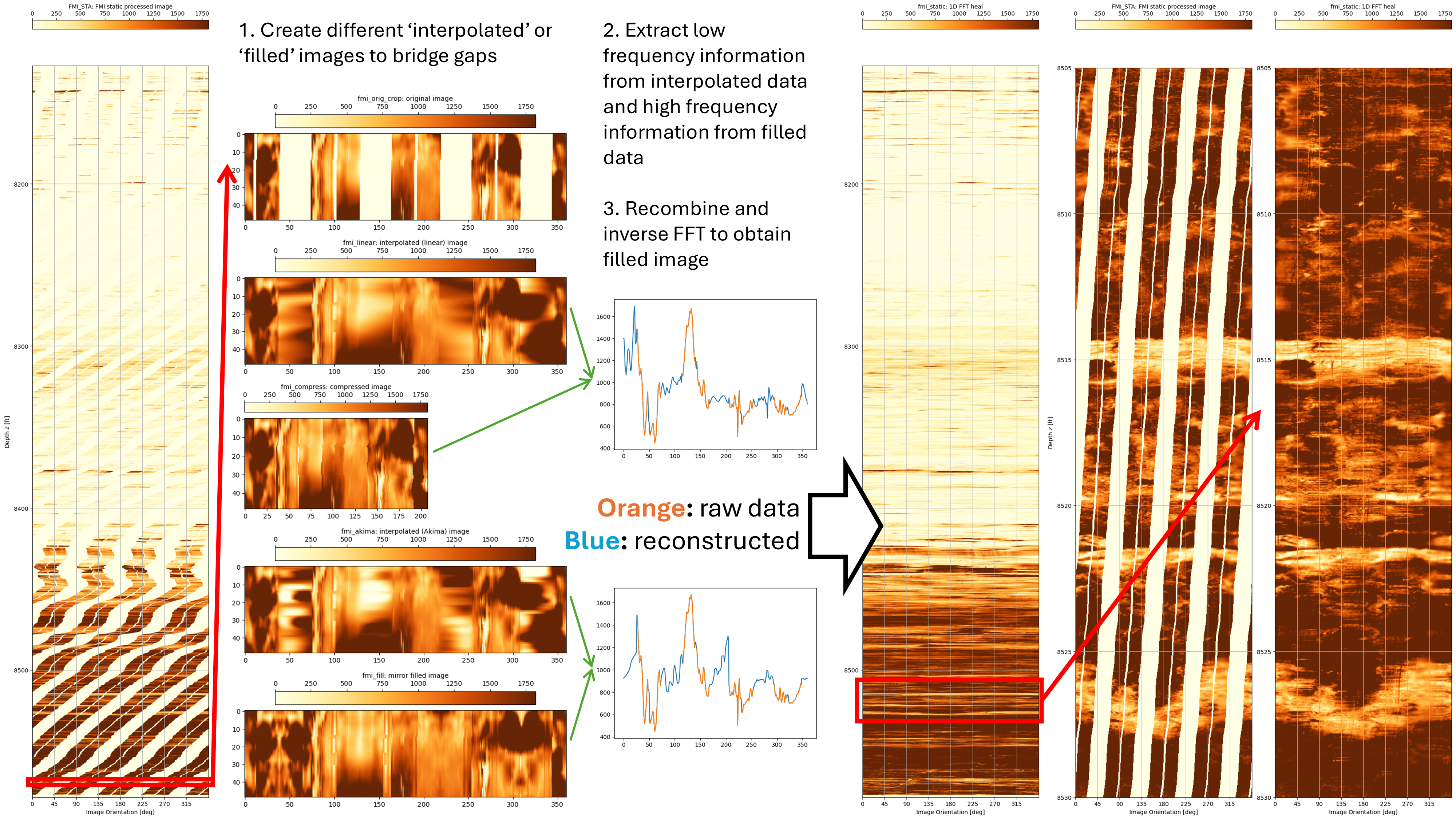
Since most of this post is quite technical in nature, and almost certainly of no interest to most people, the TLDR (too long, didn’t read) summary can be seen in the Figure below.
Evidently dlisio is a useful and workable solution for reading FMI logs. The next challenge is how to incorporate this library into the Pyrus Suite which is written in Java. dlisio is an open-source library hosted on GitHub which means the source could be examined and then ported to Java. However, it appears that the Python library actually wraps an underlying C++ core, the source code for which is not published. One approach might be to re-wrap the exposed methods using SWIG and then call these in Java. An alternative approach could be to use GraalPy which is an implementation of the Python language that runs on the Java Virtual Machine. There may be other approaches that I haven’t come across yet, although I suspect whatever route is taken, it is going to be slow and arduous.
Part 1: Open a DLIS File Using dlisio
Import dlisio module and needed libraries
The first step is to import Equinor’s dlisio module into this Jupyter notebook environment. This module wraps a C++ core with a Python interface, and allows the DLIS files to be read. Once dlisio has been imported, we then also import other packages that we need to interact with the file.
# Install a pip package in the current Jupyter kernel
import sys
!{sys.executable} -m pip install dlisio

# Import libraries (Jupyter knows about these libraries so a special import is not required)
from dlisio import dlis
from tqdm import tqdm
import math
import pandas as pd
import numpy as np
import matplotlib.pyplot as plt
import ipywidgets as widgets
from IPython.display import display
from scipy import interpolate
from scipy import ndimage

# Ensure that we can see pandas tables of up to 1000 rows as DLIS parameter lists can be very long
pd.set_option('display.max_rows', 1000)
Define the DLIS files
There are two types of DLIS file available. The raw DLIS recorded by the FMI tool, and processed DLIS logs which contain processed logs for the static and dynamic images. These files are located in the same folder as this Jupyter notebook and can be read in directly using dlisio.
First we will check that the files exist and display some information about what is contained within each.
- Check that our Pasca A FMI log can be found.
- Print out the description of all logical files contained within each DLIS file.
filenames = []
filenames.append("Pasca A4(AD-1) Schlumberger FMI (Main Pass 8,131'-8,577') DLIS.dlis")
filenames.append("Pasca_A4(AD-1)_SLB_S2R8_FMI_MainPass_Static_Processed_Image_data.dlis")
filenames.append("Pasca_A4(AD-1)_SLB_S2R8_FMI_MainPass_Dynamic_Processed_Image_data.dlis")
import os.path
for fn in filenames:
    print(fn)
    print(os.path.exists(fn))
Pasca A4(AD-1) Schlumberger FMI (Main Pass 8,131'-8,577') DLIS.dlis
True
Pasca_A4(AD-1)_SLB_S2R8_FMI_MainPass_Static_Processed_Image_data.dlis
True
Pasca_A4(AD-1)_SLB_S2R8_FMI_MainPass_Dynamic_Processed_Image_data.dlis
True
The files are found in the working directory and can now be passed to dislio to load the data. First we will examine the structure of the files.
for fn in filenames:
    with dlis.load(fn) as files:
        print('Data contained in file: "', fn, '"\n')
        for f in files:
            print(f.describe())
Data contained in file: " Pasca A4(AD-1) Schlumberger FMI (Main Pass 8,131'-8,577') DLIS.dlis "

------------
Logical File
------------
Description : LogicalFile(ConCu_R09_L002Up_FBST_HNGC_HNGS_HGNS)
Frames      : 4
Channels    : 8

Known objects
--
FRAME       : 4
CHANNEL     : 8
FILE-HEADER : 1
PARAMETER   : 339
ORIGIN      : 5


------------
Logical File
------------
Description : LogicalFile(EID)
Frames      : 1
Channels    : 7

Known objects
--
FRAME       : 1
TOOL        : 1
CHANNEL     : 7
FILE-HEADER : 1
PROCESS     : 1
PARAMETER   : 366
ORIGIN      : 2


Data contained in file: " Pasca_A4(AD-1)_SLB_S2R8_FMI_MainPass_Static_Processed_Image_data.dlis "

------------
Logical File
------------
Description : LogicalFile(EID)
Frames      : 1
Channels    : 21

Known objects
--
FRAME       : 1
TOOL        : 1
CHANNEL     : 21
FILE-HEADER : 1
PROCESS     : 1
PARAMETER   : 366
AXIS        : 2
ORIGIN      : 2


Data contained in file: " Pasca_A4(AD-1)_SLB_S2R8_FMI_MainPass_Dynamic_Processed_Image_data.dlis "

------------
Logical File
------------
Description : LogicalFile(EID)
Frames      : 1
Channels    : 21

Known objects
--
FRAME       : 1
TOOL        : 1
CHANNEL     : 21
FILE-HEADER : 1
PROCESS     : 1
PARAMETER   : 366
AXIS        : 2
ORIGIN      : 2
It can be seen that each DLIS file contains logical files, each of which in turn contain “frames” and “channels”. The immediate question I had was, “so where is the data”? Is it in a frame or a channel? What are the parameters?
More information on the DLIS format (RP66 V1) specification was originally proposed to the American Petroleum Institute (API) by Schlumberger and then passed to the Petrotechnical Open Software Corporation (POSC) in June 1998. In the Pyrus suite I’ve written code to read and write SEG-Y seismic data, LAS well log data, a lexer/parser fro the ECLIPSE reservoir simulation language, code to translate between different raster image formats such as TIFF, PNG, JPG, Vidar Binary (very obscure) etc. I look at the DLIS specification and my first thought is, “but why”?! Suffice to say it feels like a sledgehammer looking for a nail where a simple flathead screwdriver would have been fine.
Additional information
The first logical file (“Pasca A4(AD-1) Schlumberger FMI (Main Pass 8,131’-8,577’) DLIS.dlis”) lists five origins for the first logical file. The next two files (“Pasca_A4(AD-1)_SLB_S2R8_FMI_MainPass_Static_Processed_Image_data.dlis” and “Pasca_A4(AD-1)_SLB_S2R8_FMI_MainPass_Dynamic_Processed_Image_data.dlis”) contain two origins each. If we have more than one logical file and one origin, we need to be careful that the data is associated with the same well. We can see here that this is the case for the raw data which lists “/ PascaA4(AD-1)” for all origins. Note that in the interests of brevity, the output of the origins after the first two have been truncated.
with dlis.load(filenames[0]) as files:
    for f in files:
        for o in f.origins:
            print(o.describe())
------
Origin
------
name   : WELL-PascaA4(AD-1)
origin : 98
copy   : 0

Logical file ID          : ConCu_R09_L002Up_FBST_HNGC_HNGS_HGNS
File set name and number : CONCU_R09_L002UP_FBST_HNGC_HNGS_HGNS / 1
File number and type     : 0 / CUSTOMER

Field                   : Pasca A
Well (id/name)          :  / PascaA4(AD-1)
Produced by (code/name) : 440 / Schlumberger
Produced for            : Twinza Oil PNG Ltd
Created                 : 2017-12-15 18:16:02

Created by              : Techlog, (version: 2017.1 (rev: 210977))
Other programs/services : WELL-PascaA4(AD-1)


------
Origin
------
name   : DATASET-FMI_8_GF_2477-2614m_New_Img_Dynamic
origin : 99
copy   : 0

Logical file ID          : ConCu_R09_L002Up_FBST_HNGC_HNGS_HGNS
File set name and number : CONCU_R09_L002UP_FBST_HNGC_HNGS_HGNS / 1
File number and type     : 0 / CUSTOMER

Field                   : Pasca A
Well (id/name)          :  / PascaA4(AD-1)
Produced by (code/name) : 440 / Schlumberger
Produced for            : Twinza Oil PNG Ltd
Created                 : 2017-12-15 18:16:02

Created by              : Techlog, (version: 2017.1 (rev: 210977))
Other programs/services : DATASET-FMI_8_GF_2477-2614m_New_Img_Dynamic

... etc. ...
Load the processed FMI DLIS logs
To begin with we won’t worry about the raw DLIS structure. Let’s load the DLIS logs into a file array such that the static log is f[0] and the dynamic log is f[1].
# Load our two processed FMI DLIS logs
file = []
f, *tail = dlis.load(filenames[1])
lf, *tail = dlis.load(filenames[1])
file.append(lf)
lf, *tail = dlis.load(filenames[2])
file.append(lf)
Our next step is to find where the data resides within the DLIS file. To do this we need to look into the DLIS file and examine its structure and contents.
Examine the data
Define a utility method that will simply assemble all variables associated with an object into a table and list them using a pandas DataFrame. This is useful to quickly see what data is in the file.
def summarize(objs, **kwargs):
    """
    Create a pd.DataFrame that summarizes the content of 'objs', one object per row.

    Parameters
    ----------

    objs : list()
        list of metadata objects

    **kwargs
        Keyword arguments
        Use kwargs to tell summarize() which fields (attributes) of the objects you want to include in the DataFrame.
        The parameter name must match an attribute on the object in 'objs', while the value of the parameters is used
        as a column name. Any kwargs are excepted, but if the object does not have the requested attribute, 'KeyError'
        is used as the value.

    Returns
    -------

    summary : pd.DataFrame
    """
    summary = []
    for attr, label in kwargs.items():
        column = []
        for obj in objs:
            try:
                value = getattr(obj, attr)
            except AttributeError:
                value = 'KeyError'
            except ValueError:
                value = 'Array'
            column.append(value)
        summary.append(column)
    summary = pd.DataFrame(summary).T
    summary.columns = kwargs.values()
    return summary
List out parameters
There are 339 parameters for our static DLIS log, and in the interests of brevity not all are shown in this post. Here the summarize method is a utility method that assembles all variables associated with an object into a table and lists them using a pandas DataFrame, as shown in the previous section. Because there are so many parameters, we filter them to a selected few so that we can see their values.
desc_parameters = ['CN', 'WN', 'FN',                                     # Well ID
                   'LOND', 'LATD',                                       # Well location
                   'DLAB', 'TLAB']                                       # Time and date of well logging

# Create a table out of the parameters in desc_parameters
parameter_table = summarize(file[0].parameters, name='Name', long_name='Long name', values='Value(s)')
desc_table = parameter_table.loc[parameter_table['Name'].isin(desc_parameters)].copy()

# Sort the table in the same order as desc_parameters
categorical_sorter = pd.Categorical(desc_parameters, desc_parameters, ordered=True)
desc_table['Name'] = desc_table['Name'].astype(categorical_sorter.dtype)
desc_table.sort_values(by='Name', inplace=True)

# Display the table
display(desc_table)
| Name | Long name | Value(s) | |
|---|---|---|---|
| 272 | CN | Company Name | [Twinza Oil PNG Ltd] |
| 111 | WN | Well Name | [PascaA4(AD-1)] |
| 264 | FN | Field Name | [Pasca A] |
| 296 | LOND | Longitude | [144.9091033935547] |
| 69 | LATD | Latitude (N=+ S=-) | [-8.596839904785156] |
| 33 | DLAB | Date Logger At Bottom | [30-Nov-2017] |
| 67 | TLAB | Time Logger At Bottom | [10:58:31] |
This shows that the parameters for the DLIS file contain data about the logging run (essentially the information typically included in a log header at the top of a well log).
List out channels
So if the FMI data values are not in the parameters, they are probably hiding somewhere in the channels. We need to know what channels area available in each of the frames. First we can iterate over all the frames in each of our static and dynamic files and show the depth ranges and channels available.
for f in file:
    for frame in f.frames:

        # Search through the channels for the index and obtain the units
        for channel in frame.channels:
            if channel.name == frame.index:
                depth_units = channel.units

        print(f'Frame Name: \t\t {frame.name}')
        print(f'Index Type: \t\t {frame.index_type}')
        print(f'Depth Interval: \t {frame.index_min} - {frame.index_max} {depth_units}')
        print(f'Depth Spacing: \t\t {frame.spacing} {depth_units}')
        print(f'Direction: \t\t {frame.direction}')
        print(f'Num of Channels: \t {len(frame.channels)}')
        print(f'Channel Names: \t\t {str(frame.channels)}')
        print('\n')
Frame Name: 		 B34276
Index Type: 		 BOREHOLE-DEPTH
Depth Interval: 	 8127.008333333333 - 8578.533333333327 ft
Depth Spacing: 		 -0.008333333333333226 ft
Direction: 		 DECREASING
Num of Channels: 	 21
Channel Names: 		 [Channel(TDEP), Channel(ASSOC_CAL), Channel(BS), Channel(C1), Channel(C2), Channel(DEVI), Channel(FLAP_1), Channel(FLAP_2), Channel(FLAP_3), Channel(FLAP_4), Channel(FMI_STA), Channel(GR), Channel(HAZI), Channel(P1AZ), Channel(P1NO), Channel(PAD_1), Channel(PAD_2), Channel(PAD_3), Channel(PAD_4), Channel(RB), Channel(SDEV)]


Frame Name: 		 B34276
Index Type: 		 BOREHOLE-DEPTH
Depth Interval: 	 8127.008333333333 - 8578.533333333327 ft
Depth Spacing: 		 -0.008333333333333226 ft
Direction: 		 DECREASING
Num of Channels: 	 21
Channel Names: 		 [Channel(TDEP), Channel(ASSOC_CAL), Channel(BS), Channel(C1), Channel(C2), Channel(DEVI), Channel(FLAP_1_DYN), Channel(FLAP_2_DYN), Channel(FLAP_3_DYN), Channel(FLAP_4_DYN), Channel(FMI_DYN), Channel(GR), Channel(HAZI), Channel(P1AZ), Channel(P1NO), Channel(PAD_1_DYN), Channel(PAD_2_DYN), Channel(PAD_3_DYN), Channel(PAD_4_DYN), Channel(RB), Channel(SDEV)]
This reveals that there are 21 channels, and their names, each in frame B34276 for the static FMI and dynamic FMI files. Data is from 8,127.0083 ft to 8,578.5333 ft, in 0.0083 ft intervals. This is 120 intervals per foot, or 0.1 inch per depth interval. This is a much higher resolution than typical wireline logging data from a triple-combo tool.
Of interest are the “FMI_STA” and “FMI_DYN” channels. Let’s take a closer look at these channels:
# Static FMI channels
channel_table = summarize(file[0].channels, name='Channel Name', units='Units', dimension='Dimension', frame='Frame')
channel_table.sort_values('Channel Name')
| Channel Name | Units | Dimension | Frame | |
|---|---|---|---|---|
| 1 | ASSOC_CAL | in | [1] | Frame(B34276) |
| 2 | BS | in | [1] | Frame(B34276) |
| 3 | C1 | in | [1] | Frame(B34276) |
| 4 | C2 | in | [1] | Frame(B34276) |
| 5 | DEVI | deg | [1] | Frame(B34276) |
| 6 | FLAP_1 | [24] | Frame(B34276) | |
| 7 | FLAP_2 | [24] | Frame(B34276) | |
| 8 | FLAP_3 | [24] | Frame(B34276) | |
| 9 | FLAP_4 | [24] | Frame(B34276) | |
| 10 | FMI_STA | [360] | Frame(B34276) | |
| 11 | GR | gAPI | [1] | Frame(B34276) |
| 12 | HAZI | deg | [1] | Frame(B34276) |
| 13 | P1AZ | deg | [1] | Frame(B34276) |
| 14 | P1NO | deg | [1] | Frame(B34276) |
| 15 | PAD_1 | [24] | Frame(B34276) | |
| 16 | PAD_2 | [24] | Frame(B34276) | |
| 17 | PAD_3 | [24] | Frame(B34276) | |
| 18 | PAD_4 | [24] | Frame(B34276) | |
| 19 | RB | deg | [1] | Frame(B34276) |
| 20 | SDEV | deg | [1] | Frame(B34276) |
| 0 | TDEP | ft | [1] | Frame(B34276) |
This shows that the “FMI_STA” channel is an array containing 360 data values for each depth interval. A similar result is obtained when inspecting the dynamic FMI data file (not shown).
Assemble the data
We now know that we are looking for channel FMI_STA in frame ‘B34276’ in the static FMI DLIS file, and for channel FMI_DYN in frame ‘B34276’ in the dynamic FMI DLIS file. There are 360 data values per depth point, which corresponds to a 360° borehole image, with one pixel per degree. Let’s now access the data associated with those channels.
First we define some utility functions to help access the correct frames and channels by name.
def get_frame(logical_file, name):
    """
    Return a frame with a given name within a logical file
    """
    [frame] = [x for x in logical_file.frames if x.name == name]
    return frame

def index_of(frame):
    """
    Return the index channel of the frame
    """
    return next(ch for ch in frame.channels if ch.name == frame.index)

def get_channel(frame, name):
    """
    Get a channel with a given name from a given frame; fail if the frame does not have exactly one such channel
    """
    [channel] = [x for x in frame.channels if x.name == name]
    return channel
Now we use the utility functions to get the data. We print out some properties to confirm we’ve got the correct data.
# Specify frames and channels to lookup
lookup_frame = ['B34276', 'B34276']
lookup_channel = ['FMI_STA', 'FMI_DYN']

# Set arrays to hold output
fmi = []
depth = []
fmi_image = []

# Iterate over the static and dynamic files
for i in range(2):

    # Get frame and its index channel
    fmi_frame = get_frame(file[i], lookup_frame[i])
    fmi_index = index_of(fmi_frame)

    # Get the metadata
    fmi.append(get_channel(fmi_frame, lookup_channel[i]))
    fmi_curves = fmi_frame.curves()
    depth.append(fmi_curves[fmi_frame.index])
    fmi_image.append(fmi_curves[lookup_channel[i]])

    # Print out the properties of the channel/curve
    print('Shape of depth index curve array: \t', depth[i].shape)
    print('Shape of FMI curve array:\t', fmi_image[i].shape)
    print(f'Name: \t\t{fmi[i].name}')
    print(f'Long Name: \t{fmi[i].long_name}')
    print(f'Units: \t\t{fmi[i].units}')
    print(f'Properties: \t{fmi[i].properties}')
    print(f'Dimension: \t{fmi[i].dimension}') #if >1, then data is an array
    print('\n')
Shape of depth index curve array: 	 (54184,)
Shape of FMI curve array:	 (54184, 360)
Name: 		FMI_STA
Long Name: 	FMI static processed image array (North orientated)
Units:
Properties: 	[]
Dimension: 	[360]


Shape of depth index curve array: 	 (54184,)
Shape of FMI curve array:	 (54184, 360)
Name: 		FMI_DYN
Long Name: 	FMI dynamic processed image array (North orientated)
Units:
Properties: 	[]
Dimension: 	[360]
We have successfully identified the data. Each static and dynamic curve contains 54,184 × 360 values. The next step is to try to plot the data so we can check that it has been read in correctly.
Plot the data
Plotting the data is achieved using matplotlib library. We first define a function to plot a curve.
def paint_channel(ax, curve, y_axis, x_axis, **kwargs):
    """
    Plot an image channel into a matplotlib axes using an index channel for the y-axis

    Parameters
    ----------

        ax : matplotlib.axes

        curve : numpy array
            The curve to be plotted

        y_axis : numpy array
            An array of values that defines the y-axis

        x_axis : numpy array
            An array of values that defines the x-axis

        **kwargs : dict
            Keyword arguments to be passed on to ax.imshow()
    """
    # Determine the extent of the image so that the pixel centres correspond with the correct axis values
    dx = np.mean(x_axis[1:] - x_axis[:-1])
    dy = np.mean(y_axis[1:] - y_axis[:-1])
    extent = (x_axis[0] - dx/2, x_axis[-1] + dx/2, y_axis[0] - dy/2, y_axis[-1] + dy/2)

    # Determine the correct orientation of the image
    if y_axis[1] < y_axis[0]:   # Frame recorded from the bottom to the top of the well
        origin = 'lower'
    else:                       # Frame recorded from the top to the bottom of the well
        origin = 'upper'

    return ax.imshow(curve, aspect='auto', origin=origin, extent=extent, **kwargs)
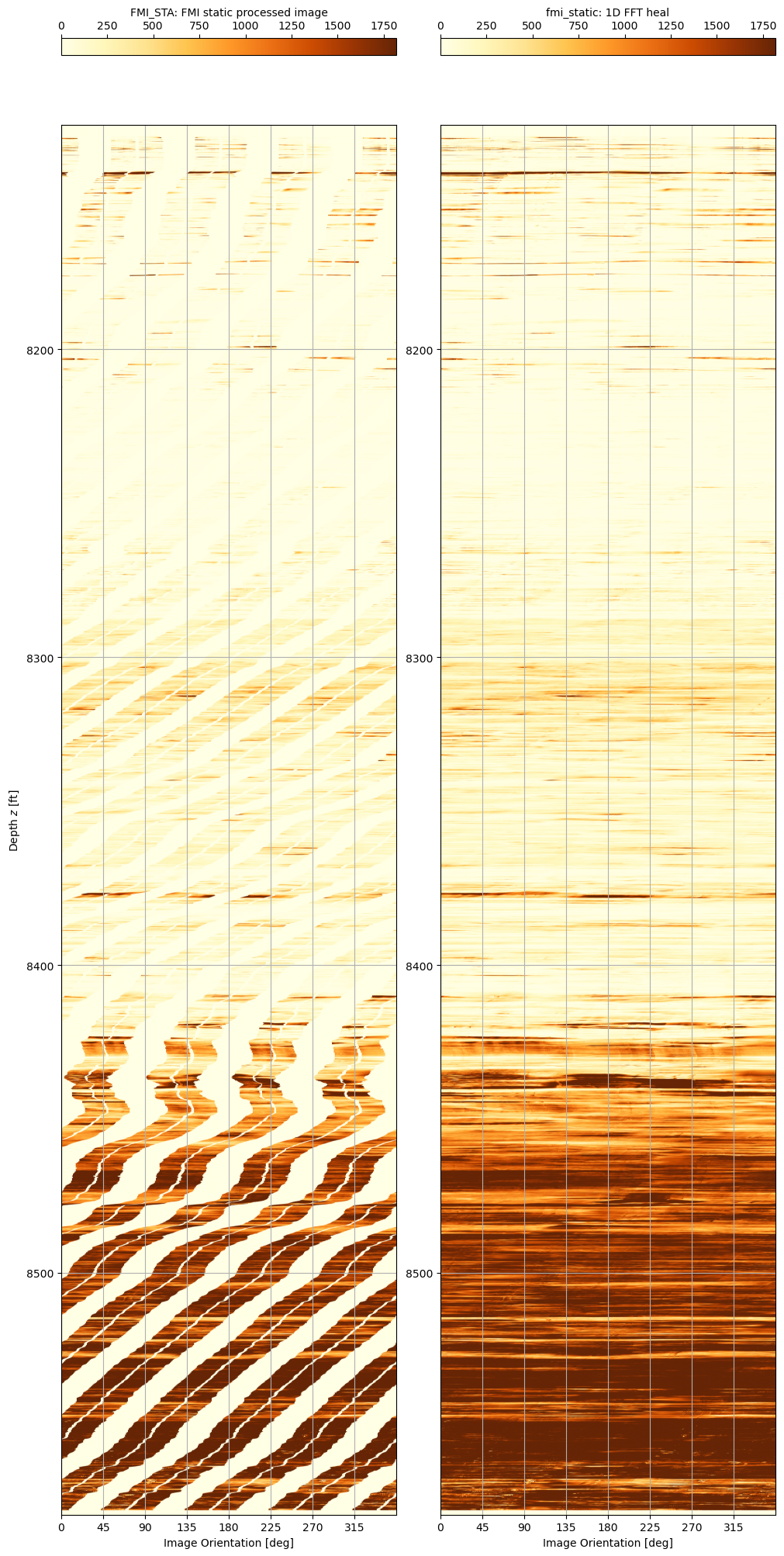
Now plot the static and dynamic images side by side using the same y-axis range. The striping of the FMI pad is clearly evident, as is the difference between the static and dynamic processed images.
def fmi_plot(MinDepth, MaxDepth, StaticFMI, DynamicFMI):

    # Determine the maximum absolute value so that we can balance the colormap maximum value
    fmi_static_max = np.percentile(np.abs(fmi_image[0]), StaticFMI)
    fmi_dynamic_max = np.percentile(np.abs(fmi_image[1]), DynamicFMI)

    # Parameters for plotting the waveforms
    fmi_static_pltargs = {
        'cmap': 'YlOrBr',
        'vmin': 0,
        'vmax': fmi_static_max,
    }
    fmi_dynamic_pltargs = {
        'cmap': 'YlOrBr',
        'vmin': 0,
        'vmax': fmi_dynamic_max,
    }

    fmi_samples = np.arange(fmi[0].dimension[0]) # x values to use in plotting

    # Create figure and axes
    fig, axes = plt.subplots(ncols=2, figsize=(10, 20), constrained_layout=True)

    # Plot static data as a colourmapped image
    ax = axes[0]
    im = paint_channel(ax, fmi_image[0], depth[0], fmi_samples, **fmi_static_pltargs)
    cbar = fig.colorbar(im, ax=ax, location='top')
    cbar.set_label(f'{fmi[0].name}: {fmi[0].long_name}')
    ax.set(ylim=[MaxDepth, MinDepth], ylabel='Depth $z$ [ft]')

    # Plot dynamic data as a colourmapped image
    ax = axes[1]
    im = paint_channel(ax, fmi_image[1], depth[1], fmi_samples, **fmi_dynamic_pltargs)
    cbar = fig.colorbar(im, ax=ax, location='top')
    cbar.set_label(f'{fmi[1].name}: {fmi[1].long_name}')
    ax.set(ylim=[MaxDepth, MinDepth])

    for ax in axes:
        ax.set(xlim=[0,360], xticks=np.arange(0, 360, 45), xlabel='Image Orientation [deg]')
        ax.grid(True)

fmi_plot(depth[0].min(), depth[0].max(), 50, 50)
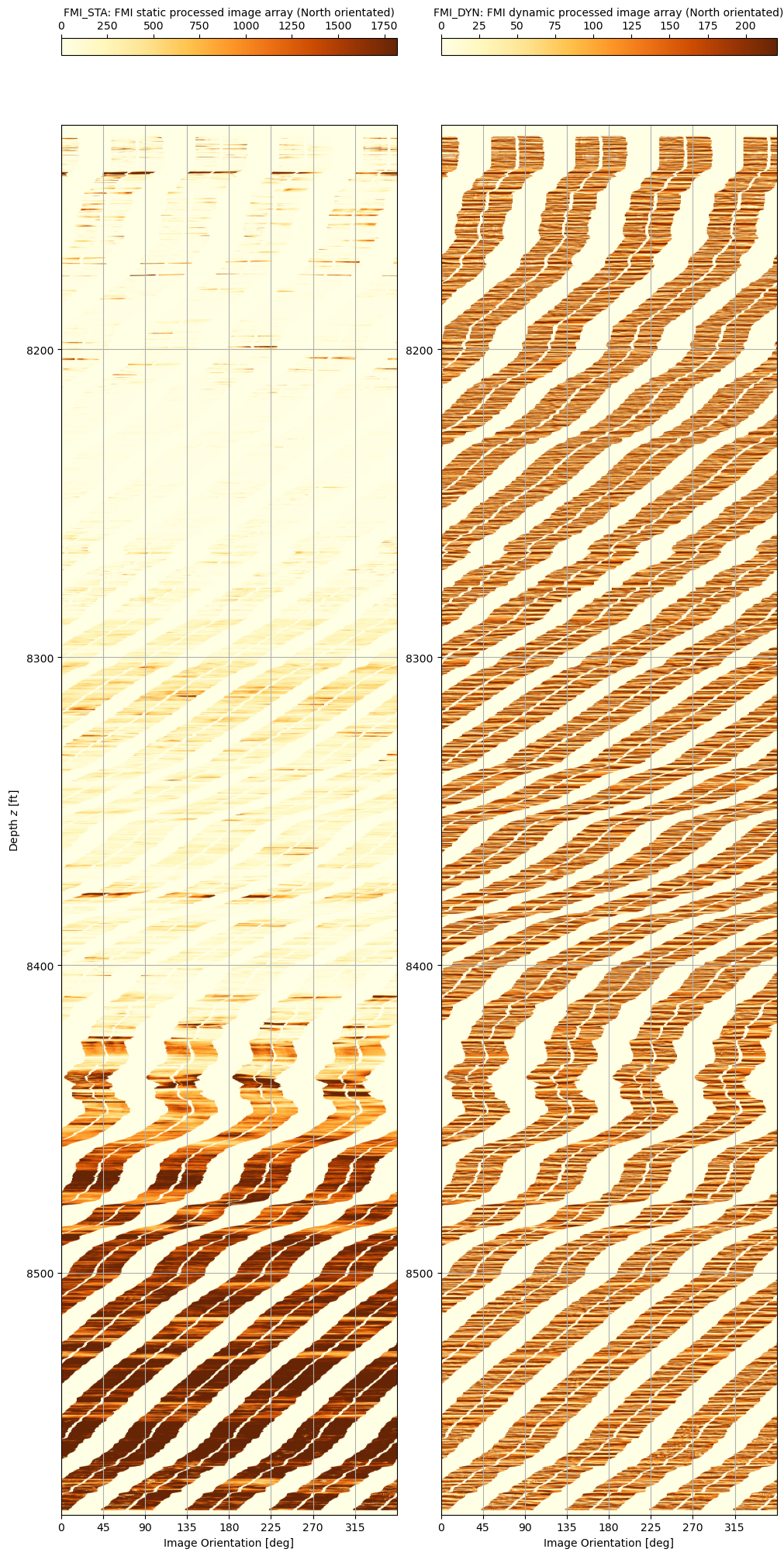
It works! The static and dynamic FMI logs can be read using dlisio. This opens the door to a whole host of different analytical techniques, including visual porosity analysis. But before we get ahead of ourselves, what can we do about the obviously striped nature of the data? The FMI tool consists of four arms that extend out and contact a pad of micro-resistivity buttons onto the borehole wall. The measurements from these buttons allow generation of a high-resolution image, but it is not continuous around the circumference of the wellbore. Perhaps it is possible to interpolate a “near enough is good enough” approximation that will trick the brain into seeing (and thus more easily comprehending) the full wellbore image?
Part 2: Experimenting to Fill Image Gaps Using Interpolation Techniques
An experimentation approach was followed to determine the algorithm to use for filling in the gaps between the pads on the FMI tool so as to create a complete borehole image. This is a sophisticated form of interpolation. The simplest brute force approach to achieve the result is simply to use linear interpolation between the pad data for each depth interval. This misses the character of the variations seen in the image (see linear interpolation sample below).
The experimental approach taken is to use the frequency data available in the data that was measured, and to then use this to fill in the gaps. We really want to preserve the overall low frequency content across the FMI image strips to provide a baseline and use the high frequency information to add detail to the missing gaps. Whilst this creates new interpolated data, it is important that the frequency and thus character of the data is preserved. The idea is that any algorithms used on the reconstructed fullbore image are not biased as a result of the reconstructed fill-in data.
A a number of test variations from our original cropped image are created:
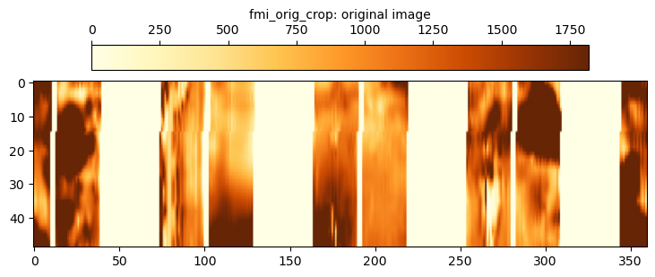
- fmi_orig_crop: This is the original static FMI data over a 0.4 ft interval down to the specified maximum depth.
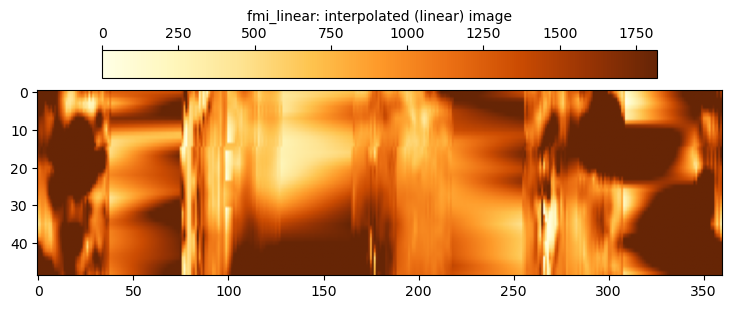
- fmi_interp: This is a basic straight line interpolation between the pad data.
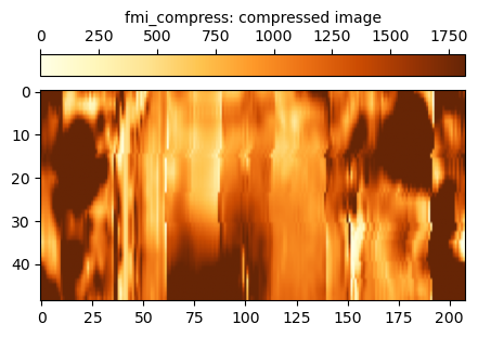
- fmi_compress: Omits the missing data and then resamples the remaining data so that it all has the same width. This contains data with the same frequencies, but because the length of the data is changed, the positional location of features would be altered.
- fmi_fill: An alternative technique which mirrors existing data into the gaps. This creates new data with (hopefully) similar or the same frequency content whilst preserving the length of the data.
# Set max depth for testing cropped image of delta_d == 0.4 ft
MaxDepth = 8570.5
MinDepth = MaxDepth - 0.4
The original fmi_orig_crop is the cropped static FMI data before any processing is applied. Note that the code used to display the cropped FMI image using matplotlib is essentially the same for all other cropped images and is not replicated following this snippet. The **fmi_static_fixpltargs variable is defined in a similar manner to the **fmi_static_pltargs variable used previous with the fmi_plot method.
# Get our cropped section for testing and show the range of index values
dint = 0.008333333333333226
d1 = int((8578.533333333327 - MaxDepth) / dint)
d2 = d1 + 49
d3 = d1 + 24
print('d1: ', d1, 'd2: ', d2, 'd3 (target row): ', d3)
fmi_orig_crop = np.copy(fmi_image[0][d1:d2, :])

# Display
nx = fmi_orig_crop[0].size
ny = len(fmi_orig_crop)
fig, axes = plt.subplots(figsize=(7.2, 3), constrained_layout=True)
im = paint_channel(axes, fmi_orig_crop, np.arange(ny)[::-1], np.arange(nx), **fmi_static_fixpltargs)
cbar = fig.colorbar(im, ax=axes, location='top')
cbar.set_label('fmi_orig_crop: original image')
The fmi_interp data uses the simplest possible approach to filling in the gaps. For each depth, a linear interpolation is applied across the gaps. It can be seen that this does successfully fill in the gaps, but the quality of the filled image is crude and does not capture any of the “texture” that is apparent in the strips themselves. It is easily discerned where the gaps were as the infill data is smooth in nature and does not contain much noise.
# Interpolate using linear method after replacing negative values with NaN (this is to get low frequencies)
fmi_linear = np.copy(fmi_orig_crop)
for j in range(ny):
    r = 0
    line = np.copy(fmi_orig_crop[j])
    while line[0] < 0 or line[nx-1] < 0:
        r -= 1
        line = np.roll(fmi_orig_crop[j], r) # roll the values so the start and end of each row are not blank
    count = 0
    for i in range(nx):
        if line[i] < 0:
            count += 1
            line[i] = np.nan
    missing_data_df = pd.DataFrame(line, columns=['value'])
    missing_data_df.interpolate(method='linear', fill_value='extrapolate', limit_direction='both', inplace=True)
    fmi_linear[j] = missing_data_df.to_numpy().flatten()
    fmi_linear[j] = np.roll(fmi_linear[j], -r) # roll back if necessary

# Display code ommitted from snippet
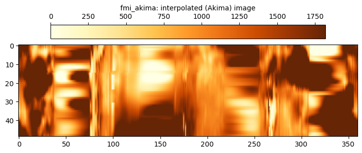
The fmi_akima data uses a more sophisticated spline interpolation approach across the gaps. A little more dynamic range appears to be captured using this approach. However, the same shortcoming as the fmi_linear approach is evident, which is that the location of the filled gap can easily be seen.
# Interpolate using Akima method after replacing negative values with NaN (this is to get low frequencies)
fmi_akima = np.copy(fmi_orig_crop)
for j in range(ny):
    r = 0
    line = np.copy(fmi_orig_crop[j])
    while line[0] < 0 or line[nx-1] < 0:
        r -= 1
        line = np.roll(fmi_orig_crop[j], r) # roll the values so the start and end of each row are not blank
    count = 0
    for i in range(nx):
        if line[i] < 0:
            count += 1
            line[i] = np.nan
    missing_data_df = pd.DataFrame(line, columns=['value'])
    missing_data_df.interpolate(method='akima', fill_value='extrapolate', limit_direction='both', inplace=True)
    fmi_akima[j] = missing_data_df.to_numpy().flatten()
    fmi_akima[j] = np.roll(fmi_akima[j], -r) # roll back if necessary

# Display code ommitted from snippet
The fmi_compress data just omits the missing gap data. This image data is used to help establish the frequencies present at each depth level. An issue with using a compressed image like this is that there are no longer 360 pixels in the x-dimension.
# Compress the image by omitting negative values
fmi_compress = []
max_len = 0
for j in range(ny):
    fmi_compress_line = []
    for val in fmi_orig_crop[j]:
        if val >= 0:
            fmi_compress_line.append(val)
    fmi_compress.append(fmi_compress_line)
    line_len = len(fmi_compress_line)
    if line_len > max_len:
        max_len = line_len

# Now resample every line to make it the same length
for j in range (ny):
    resamp_f = interpolate.interp1d(np.arange(len(fmi_compress[j])), fmi_compress[j], fill_value='extrapolate')
    fmi_compress[j] = resamp_f(np.arange(max_len))

# Display code ommitted from snippet
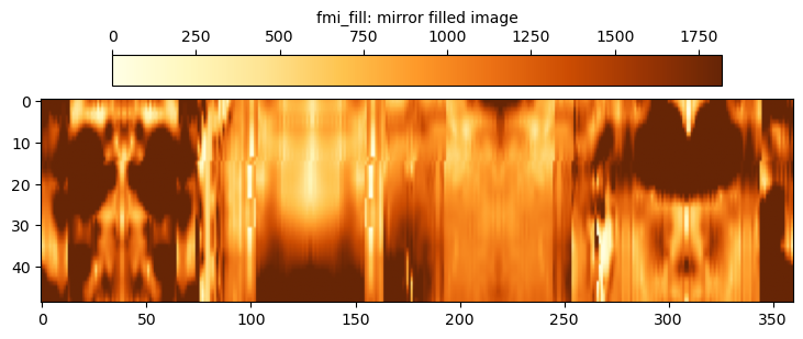
To maintain the same number of samples, an alternative approach to compressing the image is to fill in the gaps with mirrored data from the adjacent stripes. This is the fmi_fill data.
# Fill in gaps in the original cropped image using a mirroring approach
fmi_fill = []
for j in range(ny):
    r = 0
    fmi_fill_line = np.copy(fmi_orig_crop[j])
    while fmi_fill_line[0] < 0 or fmi_fill_line[nx-1] < 0:
        fmi_fill_line = np.roll(fmi_orig_crop[j], r)
        r -= 1
    i = 0
    ii = 0
    for val in fmi_fill_line:
        if val >= 0:
            i += 1
            ii = i
        else:
            idx = ii - 1
            if (idx < 0):
                idx += 360
            val = fmi_fill_line[idx]
            fmi_fill_line[i] = val
            i += 1
            ii -= 1
    fmi_fill_line = np.roll(fmi_fill_line, -r)
    fmi_fill.append(fmi_fill_line)

# Display code ommitted from snippet
Perform fast Fourier transforms to get the low frequency and high frequency components
Now that we have a technique for creating different fill-in methods, we can extract frequency data from these filled-in images and then recombine them. Generally the approach is to use the linear and Akima interpolation methods to guide the low frequency content (the absolute values) and the compressed or mirror-filled images are used to generate high frequency data that can be used to add the “noise” back into the smooth interpolated gaps. The basic principle for the proof of concept using fast Fourier transform (FFT) to fill in the gaps is as follows:
- Create fill in the gaps using a linear or Akima interpolation method.
- Perform a fast Fourier tranform on the interpolated line.
- Preserve the low frequencies from this FFT.
- Create a compressed line by omitting the gaps or a filled line by mirroring data into the gaps.
- Perform a fast Fourier transform on the compressed or filled line.
- Resample the frequencies so that they can be inverted to the same length as the original data.
- Preserve the high frequencies from this second FFT.
- Combine the low and high frequencies and perform an inverse FFT to get a new trace.
- Splice the original data and new trace so that the new trace fills the gaps in the original data.
Testing of this method reveals that the technique works and provides a quick and relatively simple way to fill in the gaps in the FMI data. Since the gaps are all in the x-direction, a 1D FFT is appropriate.
It should be possible to improve upon the method. Firstly the linear interpolation does not take into account the shape of the underlying curve where a spline-based approach might be better. The Akima interpolation method is a robust implementation that could improve the input basis for determining the low frequencies. The second shortcoming is that the frequencies in the x-direction only are considered. By using more rows above and below the target row, a 2D FFT can be considered that should improve the quality of the final inverted row, although the principle of identifying low and high frequencies and then recombining to fill in the gaps remains.
Producing a healed FMI image with no gaps
The final step is to create a single method that can be applied to a raw FMI image. Both a 1D FFT and 2D FFT approach are trialled, although the code associated with the 2D FFT method is not shown. In these tests, the 1D FFT uses linear interpolation to obtain low frequencies and extracts high frequencies from the compressed image. In comparison the 2D FFT uses the Akima interpolation to obtain low frequencies and extracts high frequencies from the mirror filled image.
def heal_fmi(fmi_orig):
    nx = fmi_orig.size

    # Unadjusted FFT of chosen row
    t = np.arange(nx)
    sp = np.fft.fft(fmi_orig)
    freq = np.fft.fftfreq(t.shape[-1])

    # Interpolate using linear method after replacing negative values with NaN (this is to get low frequencies)
    r = 0
    line = np.copy(fmi_orig)
    while line[0] < 0 or line[nx-1] < 0:
        r -= 1
        if (r < -nx):
            return fmi_orig
        line = np.roll(fmi_orig, r) # roll the values so the start and end of each row are not blank
    count = 0
    for i in range(nx):
        if line[i] < 0:
            count += 1
            line[i] = np.nan
    if count == nx:
        return fmi_orig
    missing_data_df = pd.DataFrame(line, columns=['value'])
    missing_data_df.interpolate(method='linear', fill_value='extrapolate', limit_direction='both', inplace=True)
    fmi_interp = missing_data_df.to_numpy().flatten()
    fmi_interp = np.roll(fmi_interp, -r) # roll back if necessary

    # FFT to get low frequencies
    sp_interp = np.fft.fft(fmi_interp)

    # Remove negative values which indicate there are no data (this is to get high frequencies)
    fmi_compress = []
    for val in fmi_orig:
        if val >= 0:
            fmi_compress.append(val)

    # FFT to get high frequencies and then resample
    t_compress = np.arange(len(fmi_compress))
    freq_compress = np.fft.fftfreq(t_compress.shape[-1])
    sp_compress = np.fft.fft(fmi_compress)
    resamp_f = interpolate.interp1d(freq_compress, sp_compress, fill_value='extrapolate')
    sp_compress_resamp = resamp_f(freq)

    # Combine low and high frequencies
    sp_healed = np.copy(sp_interp)
    for i in range(sp_interp.size):
        if abs(freq[i]) > 0.05 and abs(freq[i] < 0.5):
            sp_healed[i] = sp_compress_resamp[i]
    fmi_healed = np.fft.ifft(sp_healed)

    # Splice original and healed data (we don't want to overwrite the original values)
    fmi_splice = np.copy(fmi_orig)
    for i in range(nx):
        if fmi_orig[i] < 0:
            fmi_splice[i] = max(fmi_healed[i].real, 0)

    # Return our healed FMI
    return fmi_splice
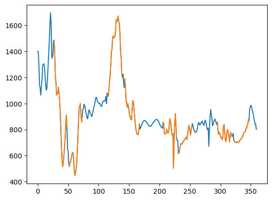
We can test the 1D FFT approach on a depth point. The line plot shows that the gap is filled continuously and preserves the character of the value variation. There appears to be a jump between the 0 and 360 degree points, so the entire circumference is not completely continuous.
test_row = 15812
print('d: ', test_row)

# Original row without negative values
fmi_nan = np.copy(fmi_image[0][test_row])
nx = fmi_nan.size
t = np.arange(nx)
for i in range(fmi_image[0][test_row].size):
    if fmi_image[0][test_row][i] < 0:
        fmi_nan[i] = np.nan

# Heal using 1D FFT
fmi_heal = heal_fmi(fmi_image[0][test_row])
plt.plot(t, fmi_heal, t, fmi_nan)
plt.show()
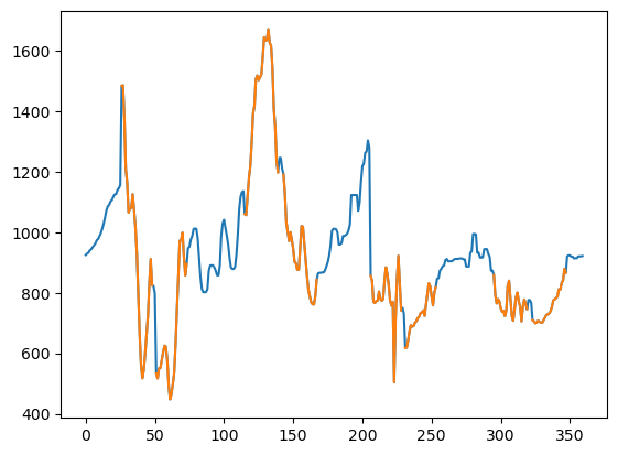
Applying the 2D approach to the same depth point shows an improvement to the circumferential continuity and there is also much better character apparent in the filled gap values, no doubt because of the 2D frequency rather than just 1D frequency data input.
test_row = 15812
d1 = test_row - 24
d2 = test_row + 25
print('d1: ', d1, 'd2: ', d2)
fmi_orig_crop = np.copy(fmi_image[0][d1:d2, :])

# Original row without negative values
fmi_nan = np.copy(fmi_image[0][test_row])
nx = fmi_nan.size
t = np.arange(nx)
for i in range(fmi_image[0][test_row].size):
    if fmi_image[0][test_row][i] < 0:
        fmi_nan[i] = np.nan

# Heal using 2D FFT
fmi_heal2 = heal_fmi2(fmi_orig_crop)
plt.plot(t, fmi_heal2[24], t, fmi_nan)
plt.show()
Applying to entire image
The heal functions are applied to the original FMI image. This process can take a while, especially for the 2D FFT which uses a 49 pixel moving window across the entire image. The 1D FFT approach is nearly two orders of magnitude faster!
fmi_static = np.copy(fmi_image[0])
ny = len(fmi_image[0])
for row in tqdm(range(ny), 'Healing FMI Image (1D FFT)'):
    fmi_static[row] = heal_fmi(fmi_image[0][row])
Healing FMI Image (1D FFT): 100%|███████████████████████████████████████████████| 54184/54184 [01:08<00:00, 792.95it/s]
fmi_static2 = np.copy(fmi_image[0])
ny = len(fmi_image[0])
for row in tqdm(range(ny), 'Healing FMI Image (2D FFT)'):
    if (row < 24):
        d1 = 0
        d2 = 49
        d3 = row
    elif (row > (ny - 24)):
        d1 = ny - 49
        d2 = ny
        d3 = 49 - (ny - row)
    else:
        d1 = row - 24
        d2 = d1 + 49
        d3 = 24
    fmi_orig_crop = np.copy(fmi_image[0][d1:d2, :])
    fmi_heal_crop = heal_fmi2(fmi_orig_crop)
    fmi_static2[row] = fmi_heal_crop[d3]
Healing FMI Image (2D FFT): 100%|██████████████████████████████████████████████| 54184/54184 [1:33:35<00:00, 9.65it/s]
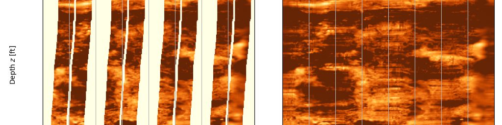
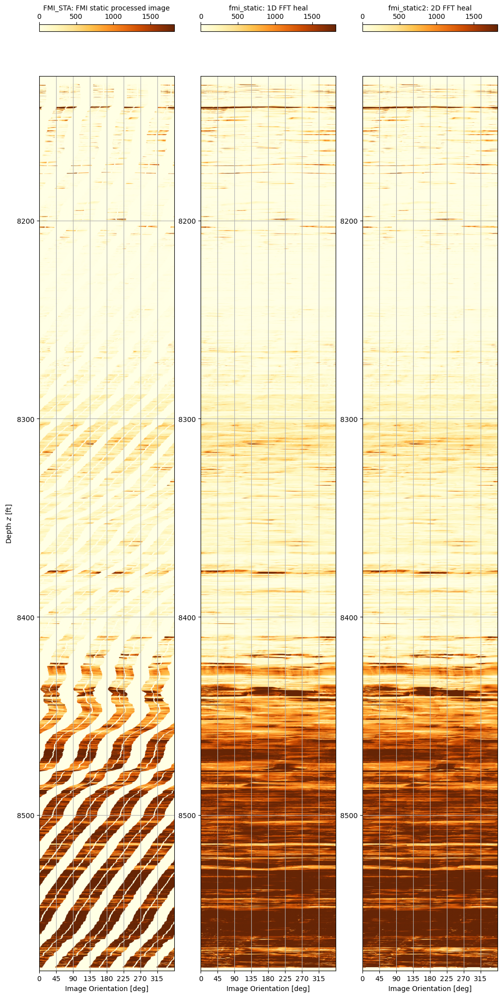
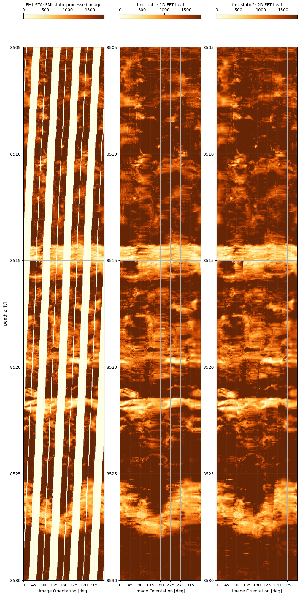
The original image and the 1D FFT and 2D FFT healed images are shown side by side. It can be seen that the 1D FFT heal process alone is quite effective. Arguably the 2D FFT healed image quality is marginally better in some aspects, but it is not a visually significant advantage. When also considering that the tradeoff is the 2D FFT approach is nearly two orders of magnitude slower, it is concluded that the 1D FFT heal algorithm is adequate. Note that the display code is similar to that used previously, and has been omitted from this blog post.
A zoom into the depth range 8,505’ to 8,530’ shows more the results of the filling techniques more clearly.
Final heal method implemented
The 1D FFT heal algorithm is a simple and relatively fast way to fill in gaps in an FMI image and in doing so, improve the ease of visualising the log image and the rock fabric texture that it represents. A downside to the method is that it does not reliably extrapolate texture features that are apparent on the FMI. In essence it is merely a sophisticated interpolation algorithm that adds noise (character) to the smooth interpolated data.
Since the 2D FFT did not offer any real improvement in image quality but was a much slower algorithm, this approach has been dropped. Instead a hybrid approach that blends both linear and Akima interpolation methods to create the low frequencies and
def heal_fmi_final(fmi_orig):
    nx = fmi_orig.size

    # Unadjusted FFT of chosen row
    t = np.arange(nx)
    sp = np.fft.fft(fmi_orig)
    freq = np.fft.fftfreq(t.shape[-1])

    # Interpolate using linear method after replacing negative values with NaN (this is to get low frequencies)
    r = 0
    line = np.copy(fmi_orig)
    while line[0] < 0 or line[nx-1] < 0:
        r -= 1
        if (r < -nx):
            return fmi_orig
        line = np.roll(fmi_orig, r) # roll the values so the start and end of each row are not blank
    count = 0
    for i in range(nx):
        if line[i] < 0:
            count += 1
            line[i] = np.nan
    if count == nx:
        return fmi_orig
    missing_data_df = pd.DataFrame(line, columns=['value'])
    missing_data_df.interpolate(method='linear', fill_value='extrapolate', limit_direction='both', inplace=True)
    fmi_linear = missing_data_df.to_numpy().flatten()
    fmi_linear = np.roll(fmi_linear, -r) # roll back if necessary

    # Interpolate using Akima method after replacing negative values with NaN (this is to get low frequencies)
    r = 0
    line = np.copy(fmi_orig)
    while line[0] < 0 or line[nx-1] < 0:
        r -= 1
        if (r < -nx):
            return fmi_orig
        line = np.roll(fmi_orig, r) # roll the values so the start and end of each row are not blank
    count = 0
    for i in range(nx):
        if line[i] < 0:
            count += 1
            line[i] = np.nan
    if count == nx:
        return fmi_orig
    missing_data_df = pd.DataFrame(line, columns=['value'])
    missing_data_df.interpolate(method='akima', fill_value='extrapolate', limit_direction='both', inplace=True)
    fmi_akima = missing_data_df.to_numpy().flatten()
    fmi_akima = np.roll(fmi_akima, -r) # roll back if necessary

    # Combine the linear and Akima interpolations
    fmi_interp = np.copy(fmi_linear)
    for i in range(fmi_linear.size):
        fmi_interp[i] *= 0.8
        fmi_interp[i] += 0.2 * fmi_akima[i]

    # FFT to get low frequencies
    sp_interp = np.fft.fft(fmi_interp)

    # Remove negative values which indicate there are no data (this is to get high frequencies)
    fmi_compress = []
    for val in fmi_orig:
        if val >= 0:
            fmi_compress.append(val)

    # FFT to get high frequencies and then resample
    t_compress = np.arange(len(fmi_compress))
    freq_compress = np.fft.fftfreq(t_compress.shape[-1])
    sp_compress = np.fft.fft(fmi_compress)
    resamp_f = interpolate.interp1d(freq_compress, sp_compress, fill_value='extrapolate')
    sp_compress_resamp = resamp_f(freq)

    # Fill in gaps in the original cropped image using a mirroring approach
    r = 0
    fmi_fill_line = np.copy(fmi_orig)
    while fmi_fill_line[0] < 0 or fmi_fill_line[nx-1] < 0:
        fmi_fill_line = np.roll(fmi_orig, r)
        r -= 1
    i = 0
    ii = 0
    for val in fmi_fill_line:
        if val >= 0:
            i += 1
            ii = i
        else:
            idx = ii - 1
            if (idx < 0):
                idx += 360
            val = fmi_fill_line[idx]
            if (val < 0):
                val = fmi_fill_line[i - 1]
            fmi_fill_line[i] = val
            i += 1
            ii -= 1
    fmi_fill_line = np.roll(fmi_fill_line, -r)

    # FFT to get high frequencies for mirror filled line and blend with compressed high frequencies
    sp_texture = np.fft.fft(fmi_fill_line)
    for i in range(sp_texture.size):
        sp_texture[i] *= 0.8
        sp_texture[i] += 0.2 * sp_compress_resamp[i]

    # Combine low and high frequencies
    sp_healed = np.copy(sp_interp)
    for i in range(sp_interp.size):
        if abs(freq[i]) > 0.05 and abs(freq[i] < 0.5):
            sp_healed[i] = sp_texture[i]
    fmi_healed = np.fft.ifft(sp_healed)

    # Splice original and healed data (we don't want to overwrite the original values)
    fmi_splice = np.copy(fmi_orig)
    for i in range(nx):
        if fmi_orig[i] < 0:
            fmi_splice[i] = max(fmi_healed[i].real, 0)

    # Return our healed FMI
    return fmi_splice

fmi_static = np.copy(fmi_image[0])
ny = len(fmi_image[0])
for row in tqdm(range(ny), 'Healing FMI Image (Final 1D FFT)'):
    fmi_static[row] = heal_fmi_final(fmi_image[0][row])
Healing FMI Image (Final 1D FFT): 100%|███████████████████████████████████████████████| 54184/54184 [02:18<00:00, 389.91it/s]
A zoom into the depth range 8,505’ to 8,530’ shows more the results of the filling techniques more clearly.
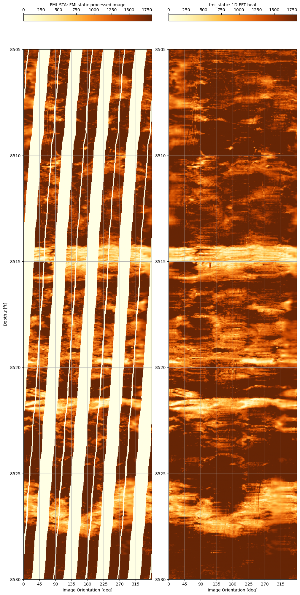
And there we have it. Formation Micro Imager data read using dlisio and gaps filled using a straightfoward merging of low frequency and high frequency data extracted from different interpolation and filling techniques.
The longer term goal is to incorporate this into Pyrus so that it can be used by others.