Viscosity governs how easily a fluid will flow and can be conceptualised as the internal fluid friction which opposes any dynamic changes to fluid flow. This makes it a very important parameter in dynamic simulation of reservoir models. Great effort has gone into understanding how viscosity can be altered to improve oil recovery, for example with thermal methods such as steam flooding that help reduce the viscosity of heavy oil and thus aid recovery.
As viscosity is the measure of internal fluid friction, it follows that the application of a shear stress on part of a fluid will impart a localised velocity to that part of the fluid. We can visualise a fluid as being made up of very small elements. Elements adjacent to the moving part of the fluid will have a frictional drag imparted onto them due to collisions between the molecules, causing them to move with a velocity that is lower than the element imparting the frictional drag. As the distance from the element onto which the original shear stress is imparted increases, the velocity decreases, leading to a velocity gradient. In addition to the elastic collisions between molecules, the inter-molecular forces (either attractive or repulsive) can also be considered.
Viscosity is defined as the local shear stress per unit area divided by the velocity gradient. Thus, for a given imposed shear stress, the lower the associated velocity gradient, the higher the viscosity. Viscosity has units of mass / (length × time) with the commonly used unit 1 Poise being equal to 1 g / (cm⋅s) or 0.1 Pa⋅s. Thus 100 cP = 1 mPa⋅s. Dynamic viscosity μ is the absolute measure of how easily a fluid will flow. It has a value of about 1.0 centipoise (cP) for water at 20 °C which makes the unit convenient to interpret. Sometimes kinematic viscosity is reported, which is simply the viscosity divided by the density (μ / ρ) and is typically shown with units of stokes (St). Note that one centistoke (cSt) is 1 cP divided by 1,000 kg/m3 which is approximately the density of water. Thus for water, the dynamic viscosity is close to 1 cP and the kinematic viscosity is close to 1 cSt.
An interesting aspect of viscosity is that it can only be measured if the fluid is moving, and is thus referred to as a non-equilibrium property. Despite this, viscosity is a function of the thermodynamic state of the fluid, and varies with temperature and pressure. Viscosity can be measured in a laboratory using a viscometer or estimated using correlations or other similar analytical methods. Note that viscosity reported in oilfield laboratory reports may not necessarily be measured as it is common to report the viscosity as calculated using a correlation.
In Pyrus, where fluid composition or type may be estimated, but actual measurements do not exist, it is necessary to implement a method to predict viscosity as accurately as possible. This assists with generation of reliable black oil tables for use in reservoir simulators. A variety of methods have been compared so as to determine the most robust and predictive approaches.
Modelling Viscosity
Whilst there are some methods for viscosity calculation that apply to both gases and liquids, in general the treatment of gases and liquids is different. In this article we cover the methods applicable to gas viscosity. Note that this article only covers in detail those methods which are not explained elsewhere in their own specific articles. Links to the more detailed articles for specific viscosity methods are included below.
Viscosity Models
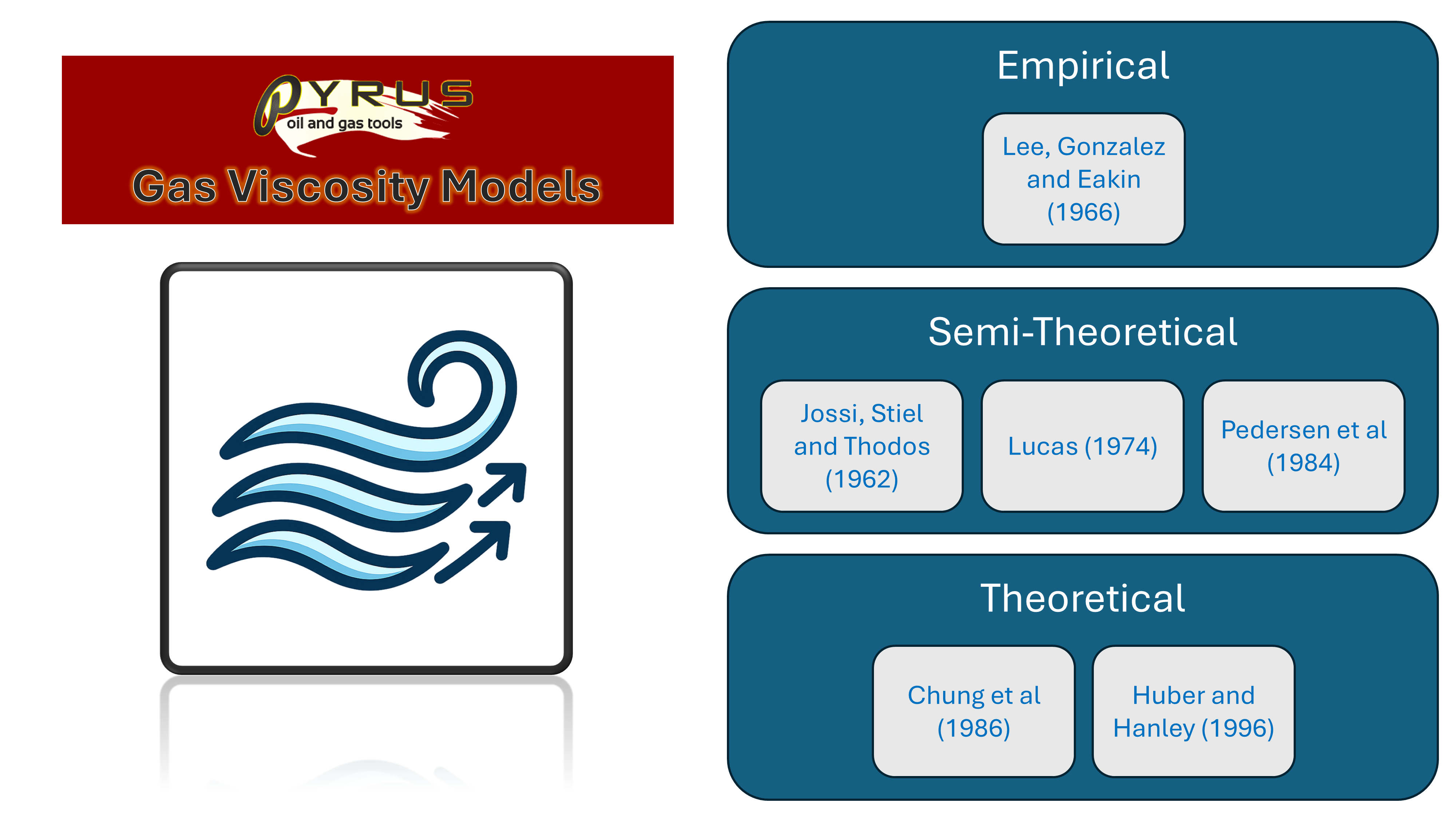
Generally there are three types of viscosity model.
- Empirical: Empirical methods are based on establishing relationships between various properties from measured datapoints. Historically these were based on statistical multi-variate regressions, but artificial neural nets are now also used. Correlations have been devised from large datasets to predict viscosity for gases and liquids against common field measurements. These approaches require that high level fluid parameters such as the gravity and saturation pressures are known. For well behaved typical oil and gas fluids, these approaches can be considered robust.
- Semi-Theoretical: Semi-theoretical models are based on theoretical principles which allow extrapolation and prediction of viscosity from first principles without use of a training dataset. These models can often be “tuned” to match experimental visosity data where it is available.
- Theoretical: Theoretical models combine effects of kinetic theory and intermolecular forces. Most approaches are based on the equations derived by Chapman and Enskog. Since this approach is based on the behaviour of interactions between colliding molecules, and the attractions (or repulsions) that exist between them, it is only applicable to modelling of gas viscosity.
In addition to the empirical versus theoretical nature of the model, there also exists a variety of different principles that are employed by gas viscosity models:
- Chapman-Enskog: Simplifications derived directly from the kinetic theory of gases and statistical mechanics. This approach calculates the intermolecular attractions and repulsions based on approximations of the relevant statistical mechanics.
- Corresponding States: Based on the principle that fluids will exhibit similar thermodynamic behaviour at the same reduced temperature and reduced pressure, it is possible to create a model for viscosity based on a known fluid and extend this to other components or mixtures. This is essentially similar to the theory of corresponding states that underpins the well-known Standing and Katz z-factor chart which uses the reduced pressure and reduced temperature to determine the z-factor. In other words, for any gas at the same conditions relative to its critical point, will exhibit similar deviation from ideal gas behaviour.
- Residual Viscosity: A relationship between the density of a fluid and its viscosity exists. The difference between the viscosity and the viscosity of the fluid at atmospheric conditions is referred to as the residual viscosity. It can be shown that values of residual viscosity plotted against density fall onto a curve, and that this appears to be independent of temperature.
- Group Contribution Techniques: Models based on group contribution methods can support predictive viscosity modelling if the composition of the fluid is known. These are typically used for low-temperature liquid viscosity approaches where corresponding states methods are less accurate. In contrast, group contribution methods take into consideration the effects of the chemical structure on viscosity.
In the oil and gas industry, both simple correlations and semi-theoretical models are the most widely used viscosity models. A common gas viscosity correlation is the Lee, Gonzalez and Eakin (LGE) model which is often used by laboratories in lieu of actual measurements. are the Lohrenz-Bray-Clark (LBC) method This is intruiging given the importance of viscosity to Darcy’s equation that governs dynamic flow. Would a more fundamental approach not be better?
The reason appears to be grounded in the use of compositional simulation models. With compositional simulation, the viscosity must be recalculated for the composition in every cell at every timestep. This can lead to millions of calculations, and thus a fast method to obtain viscosity is desirable. Whilst correlations or the LBC model may not be reliably predictive, it is possible to tune then to available laboratory measurements. This allows a fast and accurate model to be implemented where laboratory data are available to tune the model.
In contrast, the Pyrus approach attempts to be as predictive as possible with limited available data. Thus a reliable predictive method is needed to determine viscosity. A comparison between different models is discussed as a means to determine the most appropriate methods to utilise.
Correlation Models
Correlation models are a straightforward empirical approach used to predict properties from a range of input variables. Usually the input variables are known to have either a physical basis for the relationship or can be shown to be statistically significant drivers of the predicted property. This is not always the case. At the time of writing, there has been an increased interest in so-called “AI” models based on training neural nets with a dataset. When distilled down to their fundamental core methodology, it is revealed that these are no more than black-box empirical correlation methods. Whether the input variables used in such models have a physical basis or are statistically significant is not always apparent.
Gas Viscosity Correlations
Gas viscosity correlations include:
- Lee, Gonzalez and Eakin (1966): Based on the semi-empirical form of equation proposed by Starling and Ellington (1964) which itself was based on the earlier theory of viscosity presented by Born and Green (1947). This splits viscosity into a combination of kinetic and intermolecular force contributions.
- Londono (2002): Re-regression of LGE using a larger dataset.
- Sutton (2007): Adaptation of LGE specifically for gas-condensate fluids.
Often in laboratory reports the gas viscosity is not actually measured, and instead a calculated viscosity is shown. For gas fluids, a common viscosity correlation used is that of Lee, Gonzalez and Eakin (1966). The Lee, Gonzalez and Eakin (LGE) equation can be applied to both mixtures and pure components.
Improvements to this form of viscosity correlation were made by Londono et al (2002) who re-regressed the equations against a larger dataset, and Sutton (2007) who adapted the equation to account for gas-condensate fluids for which viscosity is not well predicted by the method of Lee et al. The original Lee, Gonzalez and Eakin equation can be compared to these updated versions in the form:
\[\mu_g=\mu_{gsc}\exp{[X\rho^{Y}]}\]With:
\[\mu_{gsc}=\frac{10^{-4}K}{\xi}\] \[K_{orig}=\frac{(k_1+k_2M_w)T^{k_3}}{k_4+k_5M_w+T}\] \[K_{alt}=0.807{T_{r}}^{0.618}-0.357e^{(-0.449T_{r})}+0.340e^{(-4.058T_{r})}+0.018\] \[X=x_1+\left[\frac{x_2}{T}\right]+x_3M_w\] \[Y=y_1+y_2X\]Where:
- μg = gas dynamic viscosity (cP)
- μgsc = dilute gas mixture viscosity at low (e.g. atmospheric) pressure (cP)
- Mw = molecular weight of gas mixture (lbm/lbm-mol)
- T = absolute temperature (K)
- Tr = reduced temperature \(\frac{T}{T_c}\) (dimensionless)
- Tc = critical temperature (K)
- ρ = density at temperature and pressure (g/cc)
- ξ = viscosity-reducing parameter (cP-1)
- Pc = critical pressure (atm)
Coefficients for the different forms of this correlation are given as:
| Parameter | Lee, Gonzalez and Eakin | Londono | Sutton |
|---|---|---|---|
| K | Korig | Korig | Kalt |
| ξ | 1 | 1 | \(\xi=0.9490\left(\frac{T_c}{M_w^3P_{c}^4}\right)^{1/6}\) |
| k1 | 9.379 | 16.7175 | |
| k2 | 0.01607 | 0.0419188 | |
| k3 | 1.5 | 1.40256 | |
| k4 | 209.2 | 212.209 | |
| k5 | 19.26 | 18.1349 | |
| x1 | 3.448 | 2.12574 | 3.47 |
| x2 | 986.4 | 2063.71 | 1588 |
| x3 | 0.01009 | 0.011926 | 0.0009 |
| y1 | 2.447 | 1.09809 | 1.66378 |
| y2 | -0.2224 | -0.0392851 | -0.04679 |
Implementation for LGE in Pyrus is as follows:
/**
 * Mixture viscosity using z factor and specific gravity. This uses the method of Lee, Gonzalez and Eakin (1966). It
 * is strongly recommended that the Z-factor is determined using the same specific gravity as used with this method.
 *
 * @param z the Z factor
 * @param pressure the gas pressure in psia
 * @param temperature the gas temperature in degrees Fahrenheit
 * @param sg gas specific gravity (air = 1)
 * @return the viscosity of the fluid in centiPoise
 */
public static double gasViscosityLee(double z, double pressure, double temperature, double sg) {
    double mw_gas = sg * AIR.mass();
    double rankine = temperature + 459.67;
    double a = (9.379 + 0.01607 * mw_gas) * pow(rankine, 1.5) / (209.2 + 19.26 * mw_gas + rankine) / 10000.0;
    double b = 3.448 + 986.4 / rankine + 0.01009 * mw_gas;
    double c = 2.447 - 0.2224 * b;

    // Need to calculate rho in units of g/cm^3, so different gas constant is used.
    double rho = (pressure * mw_gas) / (z * 669.95 * rankine);
    return a * exp(b * pow(rho, c));
}
Semi-Theoretical and Theoretical Models
A range of different semi-theoretical and theoretical models have been implemented in Pyrus.
Corresponding States Models
The correlation models above calculate viscosity at a given temperature and pressure. An alternative approach is to first determine the gas viscosity at a known reference condition such as atmospheric conditions, and to then adjust the reference viscosity to the target temperature and pressure. By using reduced temperature and pressure the corresponding states principle (CSP), that gas will behave similarly under the same reduced conditions, can be exploited.
Methods that are based on corresponding states include:
- Comings et al (1944): This graphical method was an early industry standard.
- Pedersen et al (1984, 1987): Uses a modified Benedict-Webb-Rubin virial equation of state for methane reference fluid together with custom mixing rules.
- Lucas (1974): Uses propane as the reference fluid together with a modification to kinetic theory to derive an equation for dimensionless viscosity as a function of reduced temperature and reduced pressure.
Comings Corresponding States Approach
Comings et al (1944) expressed the viscosity ratio as a function of the reduced pressure and reduced temperature.
\[\frac{\mu}{\mu_{1atm}}=f(p_r, T_r)\]Where:
- Pr = reduced pressure [pressure (absolute units) / critical pressure (absolute units)] (dimensionless)
- Tr = reduced temperature [temperature (absolute units) / critical temperature (absolute units)] (dimensionless)
- μ = viscosity of gas at reduced temperature Tr and reduced pressure Pr (cP)
- μ1atm = viscosity of gas at atmospheric pressure and at temperature Tr (cP)
Comings et al created various plots which allow the reduced conditions to be translated to a viscosity ratio. Carr et al (1954) extended the methodology to mixtures. In place of critical temperature and critical pressure for a component, the pseudo-critical temperature and pseudo-critical pressure for the gas mixture was obtained using Kay’s mixing rules. The dilute gas mixture viscosity was determined using the method of Herning and Zipperer (1936).
\[\mu_m=\frac{\sum_{i=1}^{n}\mu_iz_i\sqrt{M_i}}{\sum_{i=1}^{n}z_i\sqrt{M_i}}\]Where:
- μi = component dynamic viscosity (cP)
- zi = component mol fraction (dimensionless)
- Mi = component molecular weight (lbm/lbm-mol)
Until the advent of the Lee, Gonzalez and Eakin correlation, this method was often used for calculating gas viscosity by laboratories. A comparison of some measured data for pure components, binary mixtures and hydrocarbon mixtures at a range of reduced temperatures is shown in the figure below.
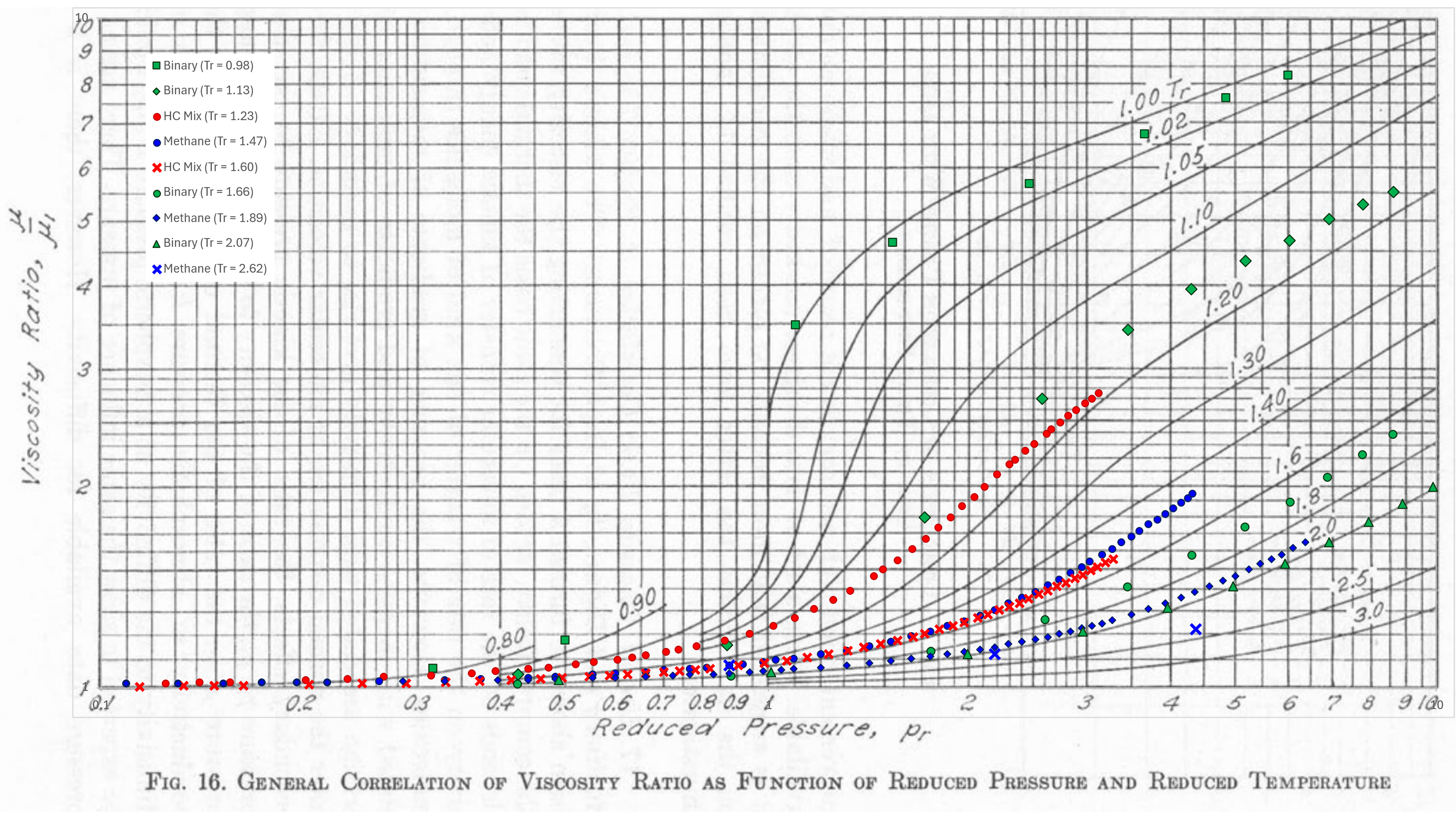
Note the limitation in the chart that only goes down to Tr = 0.8. This is because for Tr < 0.7 we are typically dealing with dense fluid viscosities (liquid viscosity).
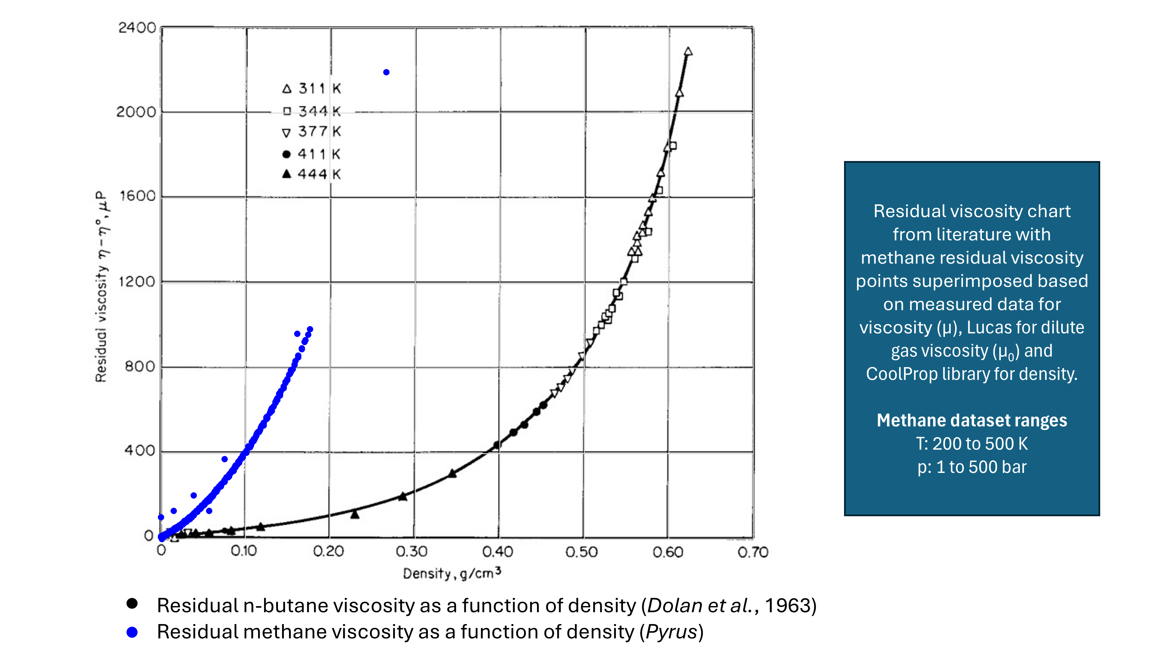
Residual Viscosity Models
Residual viscosity is defined as the difference between viscosity at a target temperature and pressure and the viscosity of the dilute gas phase (usually at 1 atm pressure and the same target temperature) = μ − μ* for pure fluids. It can be seen in Figure 3 below that a plot of residual viscosity versus density of a fluid is independent of temperature and falls on a single curve. The points shown are drawn from published literature (Dolan et al, 1963) and also generated by Pyrus based on a small test dataset of 302 methane viscosity measurements.
Methods that are based on residual viscosity include:
- Jossi, Stiel and Thodos (1962): This method is often encountered in the Lohrenz-Bray-Clark viscosity approach.
- TRAPP: The TRAnsport Properties Prediction method uses a combination of corresponding states and residual viscosity with propane as the reference fluid.
Note that the Lohrenz-Bray-Clark (LBC) correlation is often used in the oil and gas industry. Although it is not listed above, it adopts the Jossi, Stiel and Thodos (JST) method which is thus often (incorrectly) referred to as LBC. It is incorporated into almost all software packages that deal with fluid properties, not because it is necessarily the best approach, but because it is expected that the method should be available. As such it is almost universally applied. Furthermore, it is intended to calculate the viscosity of both gases and liquids, at high and low temperature and pressure. A separate article investigating the shortcomings of the Lohrenz-Bray-Clark method goes into more detail on this method. Interestingly the original procedure proposed by Lohrenz, Bray and Clark applied a different viscosity technique depending on whether the fluid is a gas or a liquid. For gases, the graphical corresponding states method of Carr et al for mixtures was applied, but with a digitised graphical chart that facilitated computerised interpolation.
Group Contribution Method Techniques
Although there are myriad equations and methods that have been developed to predict fluid viscosity, there is no universally accepted solution that accurately predicts viscosity across all fluid types. Many methods can be shown to be reasonably accurate if the pure component viscosities, or low-pressure mixture viscosity can be accurately measured. In other words, in the presence of a datapoint anchor, the principles that govern variation in viscosity with temperature and pressure are understood and viscosity at other temperatures and pressures can be reliably predicted.
But what if there is no laboratory measurement from which to ‘tune’ the viscosity model?
Group contribution methods have been successfully applied to modelling of various chemical properties, and viscosity is no exception. By breaking the molecule into smaller constituent groups, each of which contributes a certain amount to the final property through its molecular size and shape, the component viscosity can be predicted in the absence of measured data.
Techniques that are based on group contribution methods for gas viscosity include:
- Reichenberg (1975):
Reichenberg Group Contribution Method
The Reichenberg GCM method is used to determine the dilute gas viscosity of an arbitrary gas.
This is a corresponding states relation for low-pressure gas viscosity given by:
\[\mu=\frac{M^{1/2}T}{a^*\left[1+(4/T_c)\right]\left[1+0.36T_r(T_r-1)\right]^{1/6}}\frac{T_r\left(1+270\mu_r^4\right)}{T_r+270\mu_r^4}\]With:
\[a^*=\sum{n_iC_i}\]Where:
- ni = number of groups of i’th type
- Ci = group contribution as per table below
| Group | Contribution Ci |
|---|---|
| -CH3 | 9.04 |
| -CH2- | 6.47 |
| >CH- | 2.67 |
| >C< | −1.53 |
| >CH2 (Rcyc) | 6.91 |
| >CH- (Rcyc) | 1.16 |
| >C< (Rcyc) | 0.23 |
| )>CH (Raro) | 5.90 |
| )>C- (Raro) | 3.59 |
There are a total of 28 groups that are defined in the Reichenberg scheme, but only 9 are implemented in Pyrus as the focus is on hydrocarbons. A downside of the Reichenberg method is that it requires all groups to be defined. If not all groups can be determined, then Pyrus will instead fall back to the Lucas low-pressure viscosity method.
Chapman-Enskog Model
It was Maxwell who first derived a probability distribution to describe molecular velocities. Boltzmann’s equation builds on this to describe the non-equilibrium behaviour of a gas and can be used to determine how macroscopic physical quantities of a gas, such as temperature and momentum, change when a gas is in motion. From this equation it is possible to derive equations that describe transport coefficients such as viscosity in terms of molecular parameters. One such set of equations are those associated with Chapman-Enskog theory. The first-order solution for viscosity is:
\[\mu=\frac{26.69(MT)^{1/2}}{\sigma^2\Omega_v}\]Where:
- μ = gas viscosity (µP)
- M = molecular weight (g/mol)
- T = temperature (K)
- σ = hard-sphere diameter (Å)
- Ωv = viscosity collision integral
Implementations of the Chapman-Enskog model in Pyrus include:
- Chung et al (1986): Defines a relationship between the ratio of the pair-potential energy to the Boltzmann constant ε/k and the hard sphere diameter σ to solve the Chapman-Enskog equation.
References
- Ali, J. K. 1991. Evaluation of Correlations for Estimating the Viscosities of Hydrocarbon Fluids. J Pet Sci Eng 5: 351-369. https://doi.org/10.1016/0920-4105(91)90053-P.
- Born, M. and Green, H. S. 1947. A General Kinetic Theory of Liquids III: Dynamical Properties. Proc, Royal Society, London, England, 1 September, 190 (1023): 455–474. https://doi.org/10.1098/rspa.1947.0088.
- Carr, N. L., Kobayashi, R., and Burrows, D. B. 1954. Viscosity of Hydrocarbon Gases Under Pressure. J Pet Technol 6 (10): 47-55. SPE-297-G. https://doi.org/10.2118/297-G.
- Comings, E. W., Mayland, B. J., and Egly, R. S. 1944. The Viscosity of Gases at High Pressures. University of Illinois Engineering Experiment Station Bulletin No. 354.
- Chapman, S. and Cowling, T. G. 1970. The Mathematical Theory of Non-Uniform Gases, third edition. Cambridge: Cambridge University Press.
- Chung, T. H., Ajlan, M., Lee, L. L., and Starling, K. E. 1988. Generalized Multiparameter Correlation for Nonpolar and Polar Fluid Transport Properties. Ind Eng Chem Res 27: 671-679. https://doi.org/10.1021/ie00076a024.
- De Guzman, J. 1913. Relation Between Fluidity and Heat of Fusion. Anales Soc Espan Fis Y Quim 11: 353-362.
- Dolan, J. P., Starling, K. E., Lee, A. L., Eakin, B. E., and Ellington, R. T. 1963. Liquid, Gas and Dense Fluid Viscosity of n-Butane. J Chem Eng Data 8 (3): 396-399. https://doi.org/10.1021/je60018a031.
- Huber, M. L. and Hanley H. J. M. 1996. The Corresponding-States Principle: Dense Fluids. In Transport Properties of Fluids, Their Correlation, Prediction and Estimation, ed. J. Millat, J. H. Dymond, and C. A. Nieto de Castro, Chap. 12, 283-295. Cambridge: Cambridge University Press. https://doi.org/10.1017/CBO9780511529603
- Jossi, J. A., Stiel, L. I., and Thodos, G. 1962. The Viscosity of Pure Substances in the Dense Gaseous and Liquid Phases. AIChE Journal 8: 59-63. https://doi.org/10.1002/aic.690080116.
- Lee, A. L., Gonzalez, M. H., and Eakin, B. E. 1966. The Viscosity of Natural Gas. J Pet Technol 18 (8): 997-1000. SPE-1340-PA. https://doi.org/10.2118/1340-PA.
- Lohrenz, J., Bray, B. G., and Clark, C. R. 1964. Calculating Viscosities of Reservoir Fluids From Their Compositions. J Pet Technol 16 (10): 1171–1176. SPE-915-PA. https://doi.org/10.2118/915-PA.
- Londono, F. E., Archer, R. A., and Blasingame, T. A. 2002. Simplified Correlations for Hydrocarbon Gas Viscosity and Gas Density — Validation and Correlation of Behavior Using a Large-Scale Database. Paper presented at the SPE Gas Technology Symposium, Calgary, Alberta, Canada, April 2002. SPE-75721-MS. https://doi.org/10.2118/75721-MS.
- Lucas, K. 1974. Ein einfaches Verfahren zur Berechnung der Viskositat von Gasen und Gasgemischen (A Simple Method for Calculating the Viscosity of Gases and Gas Mixtures). Chem Ing Tech 46 (4): 157. https://doi.org/10.1002/cite.330460413.
- Pedersen, K. S., Christensen, P. L., and Shaikh, J. A. 2024. Phase Behavior of Petroleum Reservoir Fluids, third edition. Boca Raton: CRC Press.
- Pedersen, K. S., Fredenslund, A., Christensen, P. L., and Thomassen, P. 1984. Viscosity of Crude Oils. Chem Eng Sci 39 (6): 1011-1016. https://doi.org/10.1016/0009-2509(84)87009-8.
- Pedersen, K. S. and Fredenslund, A. 1987. An Improved Corresponding States Model for the Prediction of Oil and Gas Viscosities and Thermal Conductivities. Chem Eng Sci 42 (1): 182–186. https://doi.org/10.1016/0009-2509(87)80225-7.
- Poling, B. E., Prausnitz, J. M., and O’Connell, J. P. 2004. The Properties of Gases and Liquids, fifth edition. New York: McGraw-Hill Book Co.
- Reichenberg, D. 1975. New Methods for the Estimation of the Viscosity Coefficients of Pure Gases at Moderate Pressures (wth Particular Reference to Organic Vapors). AIChE Journal 21 (1): 181-183.https://doi.org/10.1002/aic.690210130.
- Starling, K. E. and Ellington, R. T. 1964. Viscosity Correlations for Nonpolar Dense Fluids. AIChE Journal 10: 11-15. https://doi.org/10.1002/aic.690100112.
- Stephen K. and Lucas K. 1979. Viscosity of Dense Fluids. New York: Springer. https://doi.org/10.1007/978-1-4757-6931-9.
- Sutton, R. P. 2007. Fundamental PVT Calculations for Associated and Gas/Condensate Natural Gas Systems. Paper presented at the SPE Annual Technical Conference and Exhibition, Dallas, Texas, USA, October 2005. SPE-97099-MS. https://doi.org/10.2118/97099-MS.