Kozeny-Kirkham Permeability Model

The relationship between porosity and permeability has been modelled by many different researchers. A new model is proposed based on the theoretical work of Müller-Huber, Schön, and Börner (2015) which uses a modified capillary tube model to take into account pore body and pore throat radii. The modification adds the tortuosity into the theoretical model, and derives a theoretical model that relates permeability to porosity (φ), the pore throat (r_t) and pore body (r_b) radii, and tortuosity (τ). In addition tortuosity is related to the cementation exponent (m) and the formation factor (F).

The Kozeny-Kirkham model was originally introduced as a series of short videos on LinkedIn which were based on a presentation broken down into several parts. Given the highly technical nature of some of the material, this blog post is perhaps a better medium to introduce the new model. Those videos are included in this post, along with expanded text and the original slide illustrations, and it may be useful to watch the videos if anyone is interested in learning how the Kozeny-Kirkham permeability equation was derived.

Fundamental Rock Property Relationships

Before we can start deriving our porosity-permeability relationship, I thought it would be useful to first introduce some key parameters that are used to describe the rock properties of interest. Several of these parameters can be related to each other, and those relationships are illustrated in the slides in Part I. The Pyrus Suite uses a rock model that relates rock properties to each other and allows properties to be estimated in the absence of actual data. This is useful for early stage exploration and appraisal where an understanding of reservoir flow behaviour can be extracted from geological description of the rock types. To start looking into how the Pyrus rock model works, we’ll start our journey by first considering what rock properties are of interest to us.

Part I Slides - Fundamental Rock Property Relationships

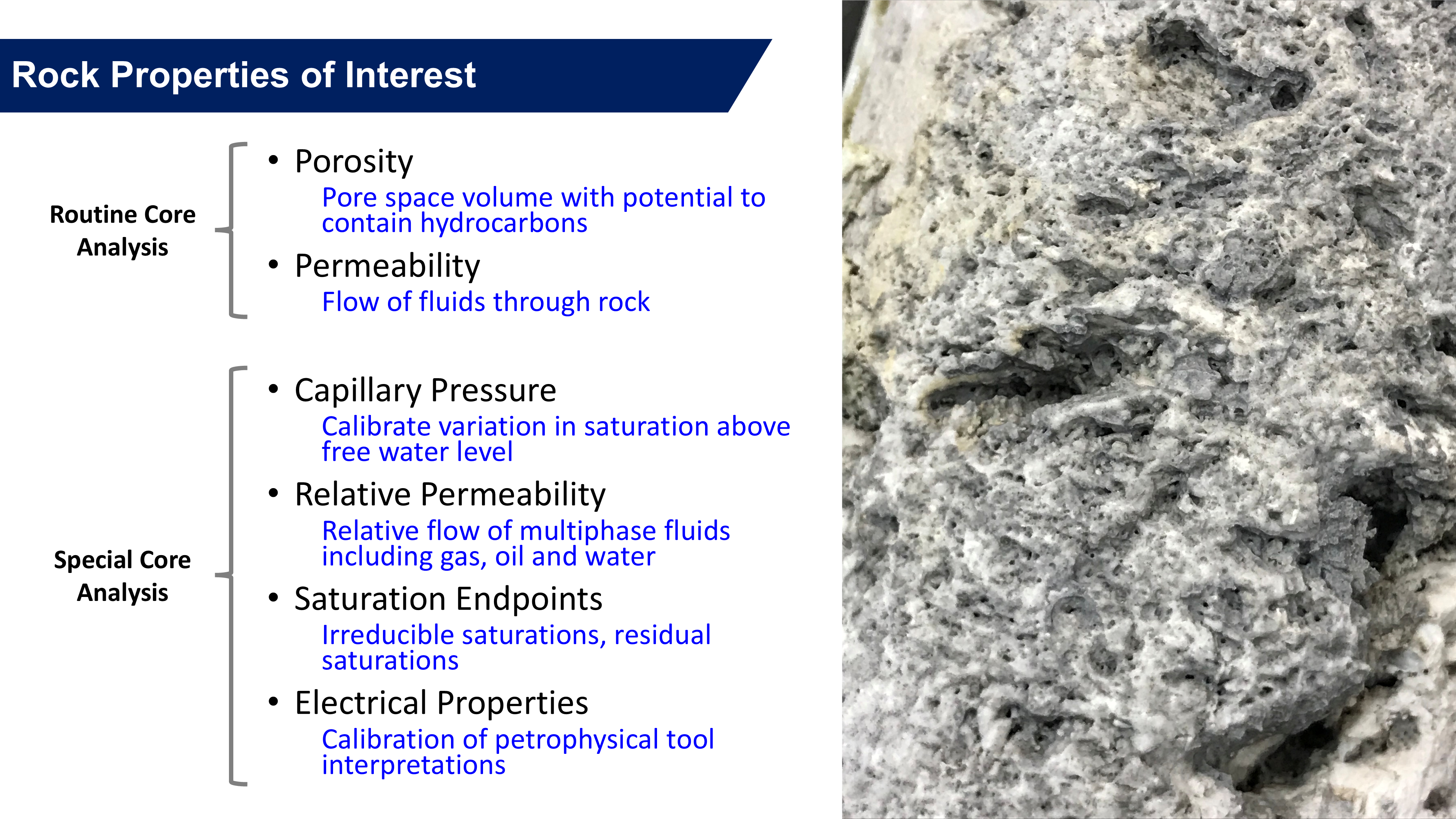
Shown in the image is a photo of carbonate take from a reef depositional environment. It can be seen that the structure is quite complex, and to describe this completely would require many different variables.

The rock properties of interest vary between different disciplines and the main properties of interest are:

• Geologists might be interested in properties such as mineralogy which provide clues as to the origin of the rock.
• Petrophysicists might be interested in properties such as grain density which can assist with log interpretation.
• Engineers are simply interested in how much fluid is in place in the rock and how easily it can be produced.
• Porosity and permeability are routinely measured on core plugs.
• Other properties are not collected as often, and special core analysis is required to measure these properties. The Pyrus rock model allows these properties to be estimated if they aren’t available.

The types of properties typically measured using routine core analysis or special core analysis are shown in Figure 1.

Let’s focus specifically on the most fundamental property which is permeability which governs how easily fluids can flow in the rock. Permeability is a complex property to understand. There are no direct permeability logging tools.

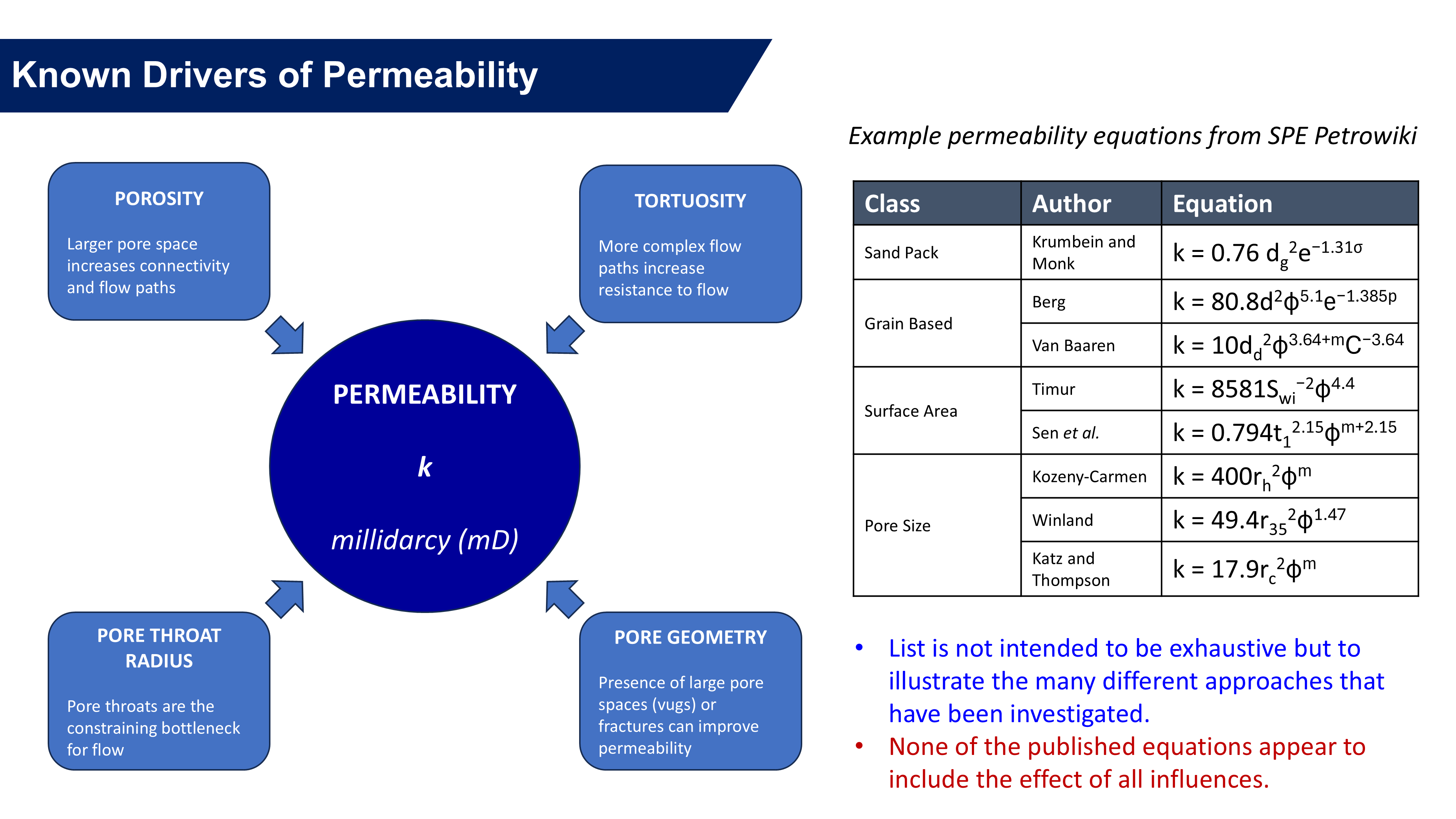
A great deal of effort has gone into understanding what controls permeability.

The four main properties that I would say have the biggest effect on permeability are shown:

1. Porosity: Larger pores means there is probably greater connectivity and wider flow paths.
2. Tortuosity: Complex flow paths through the rock increase the resistance to flow.
3. Pore throat radius: For any flow path, there will be constrictions where the pores narrow. These are the pore throats.
4. Pore geometry: It is known that large pore spaces such as vugs, or the presence of fractures can improve permeability.

These influences are shown in Figure 2.

The question is, “How do we capture this all into an equation?” Also shown on Figure 2 are a handful of example equations taken from SPE’s Petrowiki. It can be seen there are different types of equations and the parameters used vary. Many of these equations are empirical in nature, and were derived from poro-perm measurements. The point to highlight is that there are many different approaches to estimating permeability. Interestingly none of the equations seem to take into account all of the drivers of permeability.

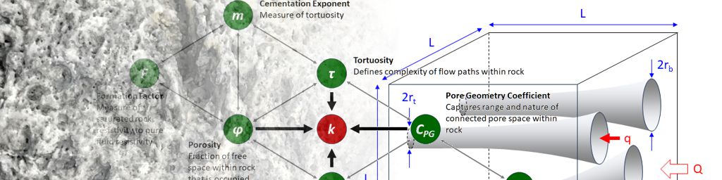
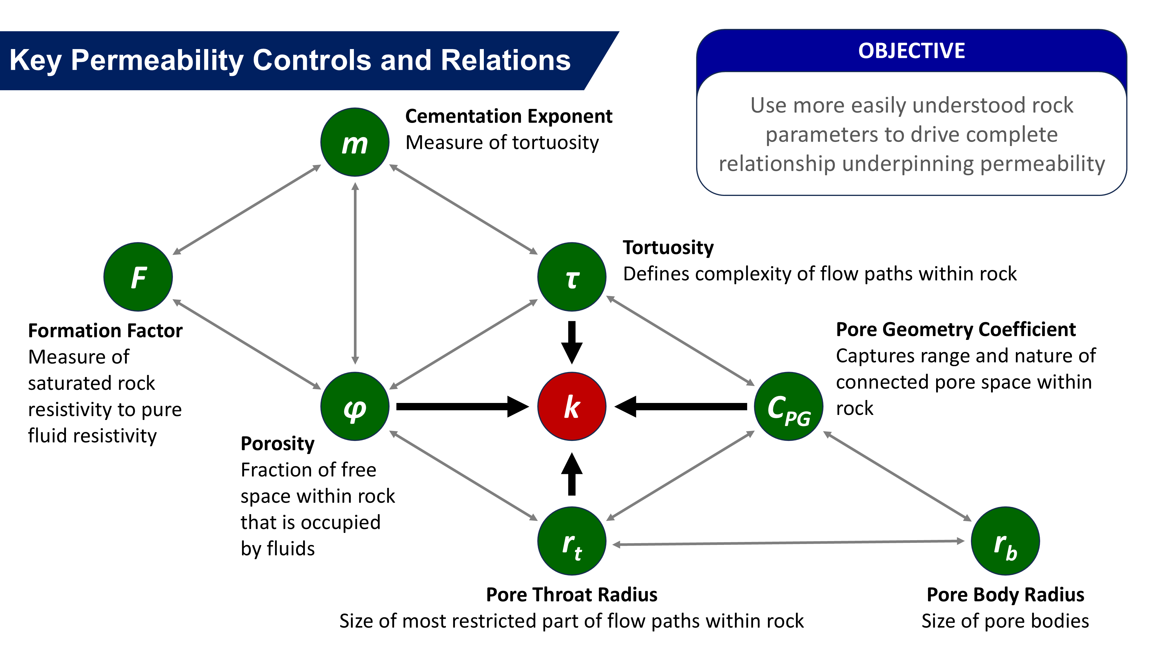
To understand the Pyrus model and approach, let’s consider the variables that control permeability. Shown on Figure 3 are various parameters and which parameters are related to each other.

Firstly there is the most fundamental relationship which are the parameters that are directly related to permeability. There is a relationship between porosity, tortuosity, the pore throat radius and the pore geometry. Together these all control permeability.

There are then a series of secondary relationships. These include the rock tortuosity which is related to the cementation exponent. The cementation exponent is itself related to the formation factor obtained by relating saturated rock resistivity to pure fluid resistivity. Finally, if we know the pore throat radius and the pore geometry, it is trivial to calculate the pore body size.

Rather than calculate or measure all the properties, the Pyrus approach involves estimating and using just a few more easily understood parameters.

Part I Video - Fundamental Rock Property Relationships

Capillary Tubes Model

So how do we actually use these parameters? First we need a solid theoretical foundation and one such model is the capillary tube model which we’ll explore in Part II. To understand the theoretical rock model that underpins Pyrus, we start by going back to basics and looking at what underpins the capillary tube model. This is amongst the simplest of rock models and has been around for many decades.

Part II Slides - Capillary Tubes Model

The capillary tubes model is deceptively simple and it is important to understand how it is derived. I have a suspicion that whilst many are aware that the Kozeny permeability model is derived from the capillary tubes model, the majority using the Kozeny equation have never actually checked by deriving it themselves.

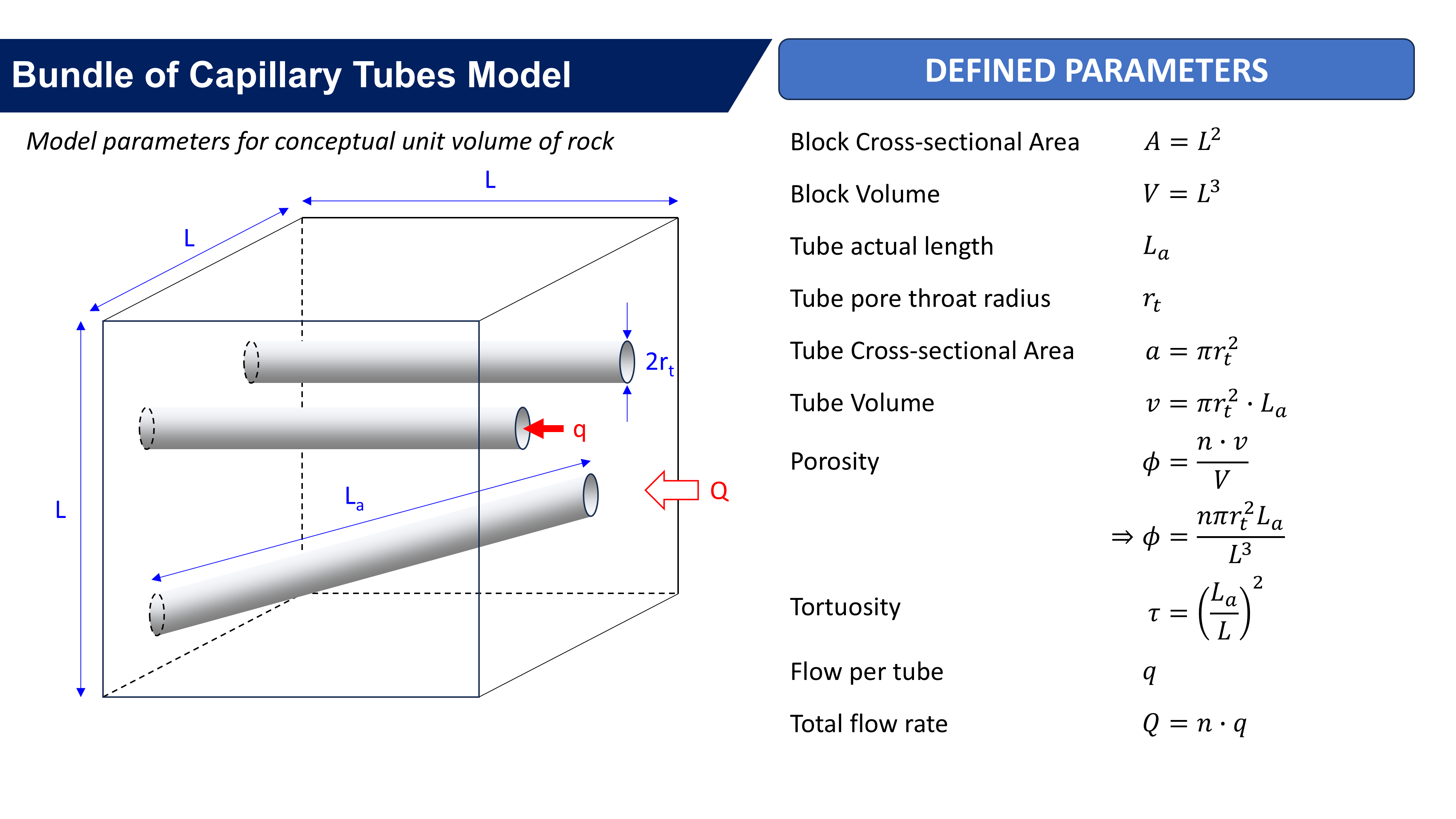
Figure 4 shows the basis for the model. A unit cube of rock matrix is penetrated by n thin tubes of constant diameter.

Let’s look at this a little closer:

• The cross-sectional area of the block is simply L².
• Multiplying by the third edge of length L gives the volume L³.
• Capillary tubes may have an internal length greater than L. We call this the actual length L_a.
• Tubes have a constant radius, which by definition must therefore be the pore throat radius r_t.

Note that longer tubes are assumed to be more like spaghetti. We assume the radius remains constant, even though the path length is longer than the length of the unit block.

From these variables alone, various properties such as volume within the tubes and thus porosity can be determined. We define tortuosity as the square of the ratio of actual length to block unit length. Finally we note that the total flow across the block is equal to the sum of individual flows through the n capillary tubes.

Let’s now calculate permeability from first principles.

The maths isn’t too hard, although it appears daunting. I wanted to spend a little time explaining the procedure here as we’ll need it later for when we change the rock model. This will change the equations, but the principles remain the same.

The two fundamental relationships we use are:

1. Darcy: This governs the flow of fluid across the gross block volume.
2. Hagan-Poiseuille: This governs the flow of fluid within an individual capillary tube.

Starting with the Darcy equation, the key observation is that the pressure differential for both the gross block flow and individual tube flow must be identical.

I walk through the steps introducing the subsitutions one at a time in the Part II video, which may be easier to follow. The steps are as follows:

1. First we substitute the pressure differential from Hagan-Poiseuille into the Darcy equation.
2. Next we substitute in known values for the previously defined block cross-sectional area and total flow.
3. q appears on both sides and can be cancelled. Then we substitute the tube cross-sectional area, a, which is based on the pore throat radius.
4. Next we must rearrange the equation to determine permeability k. Note there is a clever trick to multiply the right-hand side by \(\frac{L_aL}{L_aL}\), which is unity.
5. The benefit of this can now be seen as the form of the equation holds two more parameters: our old friends porosity and tortuosity which can be substituted in.

This leaves us with a much simpler form which is the well-known Kozeny permeability equation:

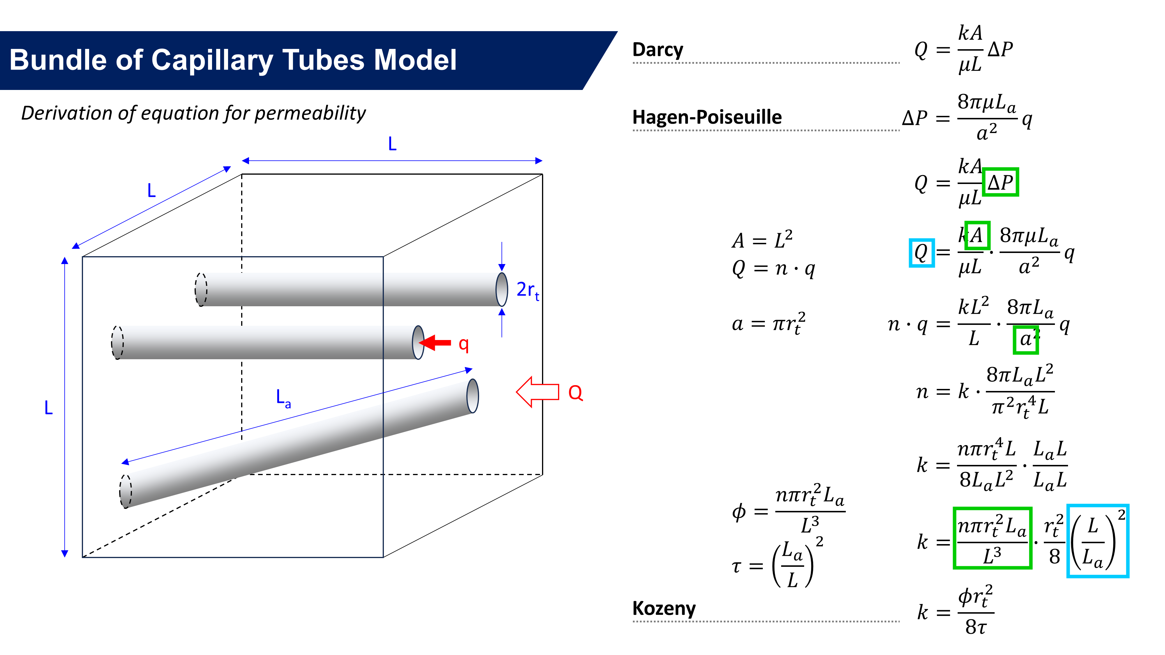
Part II Video - Capillary Tubes Model

Müller-Huber, Schön and Börner Modified Pore Throat Model

The Kozeny equation doesn’t get used much. This is perhaps because the parameters such as pore throat radius and tortuosity are much harder to estimate than the porosity. The capillary tube model is also simplification of reality.

Let’s look at a refinement to the capillary tube model instead. By making small changes to the capillary tube model we can address the simplifications, at the expense of more complex mathematical gymnastics. The model that Pyrus uses for its rock model is based on a modified pore throat model that was published by Müller-Huber, Schön and Börner (2015).

Part III Slides - Müller-Huber, Schön and Börner Modified Pore Throat Model

First let’s recall what the capillary tube model looks like. This uses a series of n thin tubes that penetrate a unit L cubed volume of rock. The biggest simplification of this model is that the capillary tubes are a constant diameter. In reality the pore network is anything but constant, with the flow path diameter changing as you move between the pore bodies themselves, and the thinner pathways (or throats) that connect them.

Let’s throw that model away and instead, let’s just make one very easy but powerful adjustment which is shown in Figure 6.

Instead of constant diameter capillary tubes, we now have variable diameter tubes. These have a notional pore body radius at one end, and a thinner pore throat radius at the other. By connecting these together, it essentially creates a model where larger pore bodies are connected via thinner and longer pore throats. This is a more realistic basis for a model.

Our parameters are almost all identical except for the tube radius. Since this is variable, it is necessary to define this using an equation r of x and then integrate along the length of a tube to get volume and hence porosity.

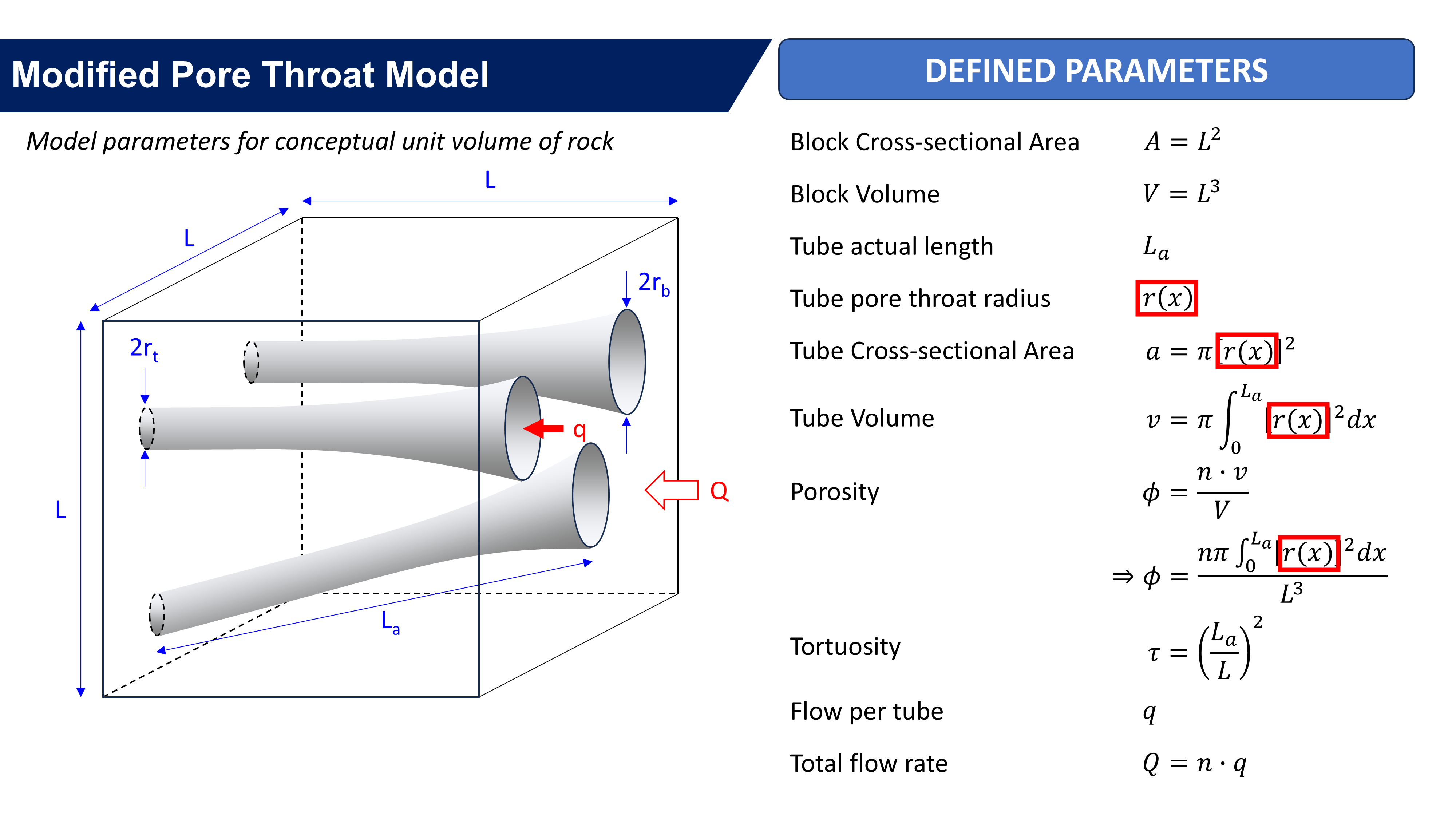
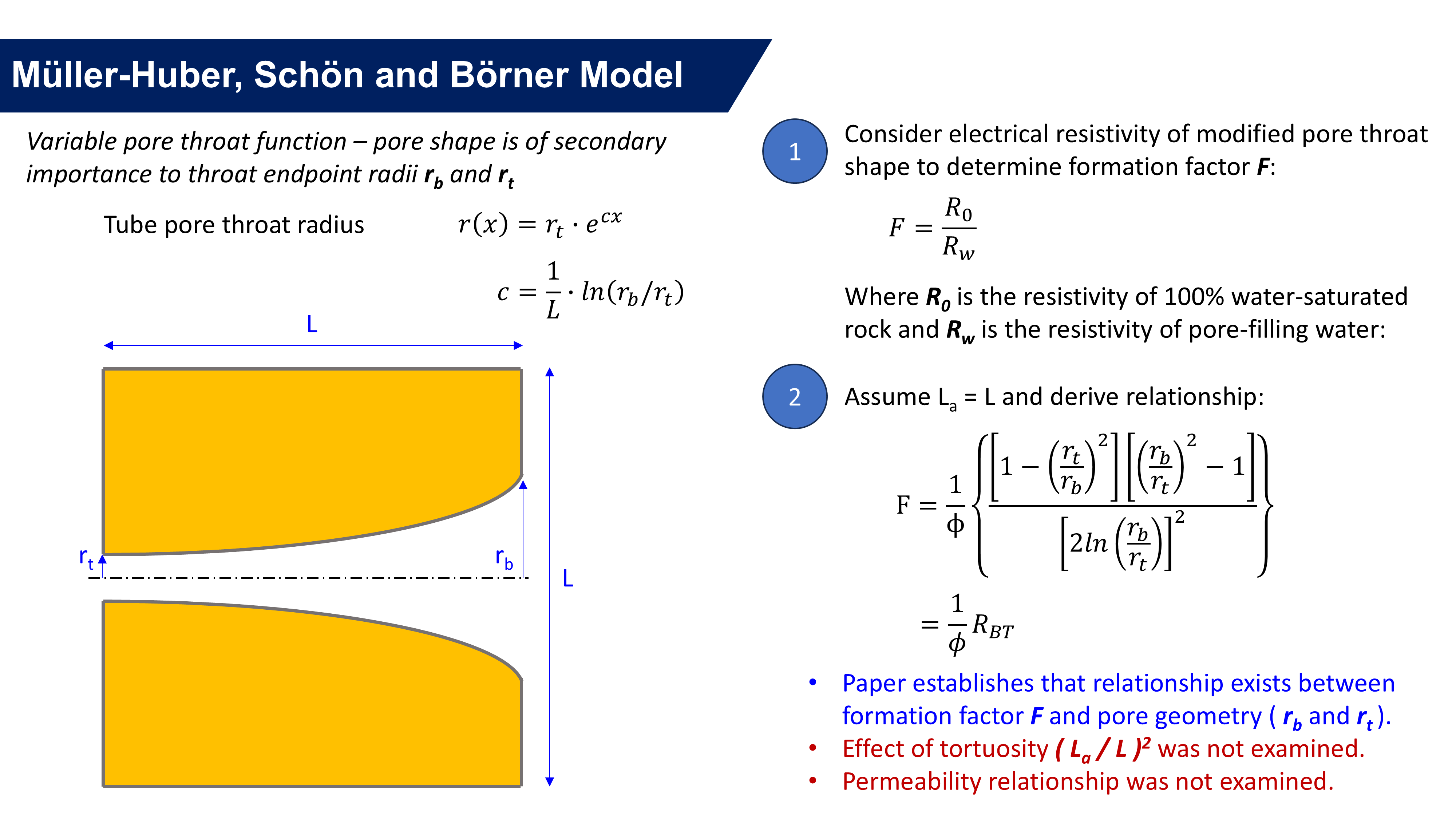
Müller-Huber, Schön and Börner were interested in using this model to improve understanding of formation factor and resistivity measurements. They define the variable pore throat radius using the equation shown in Figure 7 which creates a curve between r_t and r_b.

According to their paper, the exact equation doesn’t matter as much as the introduction of different tube radii at each end. Their analysis is based on an understanding of electrical resistivity. The presence of a rock matrix means that the conducting path for electricity follows a tortuous path through the rock and cannot conduct through the matrix itself. Thus both the porosity and the pore geometry affect the resistivity of the water-saturated rock R₀, in comparison to the resistivity of the pore-filling water R_w in the absence of a porous medium. The ratio of these two resistivities is the formation factor.

Now to simplify things assume that all the tubes are of length L. I’ll skip over the math here and jump straight to the answer, other than to quickly note for the record that I did independently verify all the equations in their paper rather than just taking them as read.

This shows the formation factor can be expressed as 1 over the porosity multiplied by a complex looking relationship involving the ratio of pore body radius to pore throat radius. We’ll define this relationship as capital R_BT or the body to throat relationship:

What their paper shows is that there is clearly a theoretical basis for a relationship between formation factor F and the pore geometry being the ratio of r_b and r_t. Of interest to our model development for permeability that will be used for Pyrus, it is noted that tortuosity was not included. And because they were looking at the effect of this model on electrical resistivity measurements, they didn’t consider permeability either. However, since flow of electrical current through pore-filling fluid along a tortuous path has a similar flow path to the actual flow of that fluid in the porous medium, there is an analogy between the two that will be demonstrated.

Part III Video - Müller-Huber, Schön and Börner Modified Pore Throat Model

Predicting Permeability with Cementation Exponent

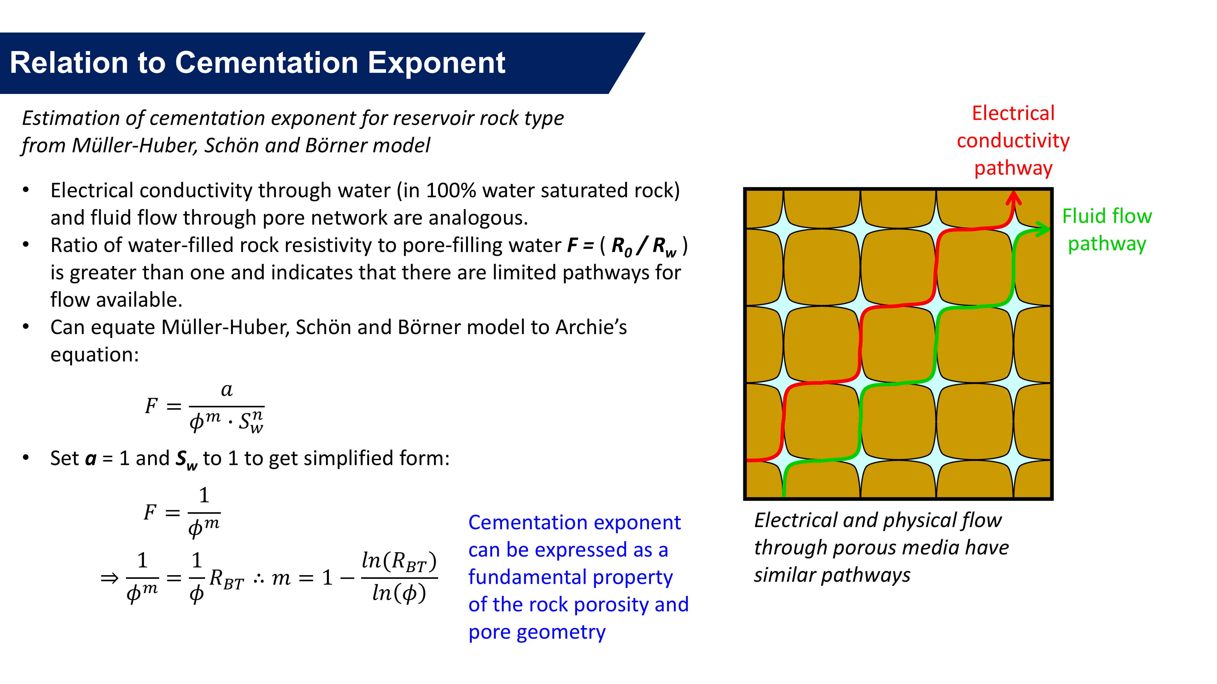
Electrical conductivity and fluid flow through a porous media are analogous. With a better model to understand formation factor, it should be possible to model cementation exponent and then apply this to permeability equations that use cementation exponent as an input variable.

Let’s examine some permeability relationships based on cementation exponent. The modified pore throat model allows the formation factor to be expressed in terms of the rock pore geometry. We can leverage this knowledge to get the cementation exponent and from that indirectly use the rock’s pore geometry to predict permeability.

Part IV Slides - Predicting Permeability with Cementation Exponent

Consider a cartoon representation of our rock model as shohwn in Figure 8. Note that the grains shown here have variable pore throat geometry which increase towards the pore bodies and narrow in the pore throats.

For electrical current to flow through the rock matrix, a circuitous route must be followed around the rock grains. This path is almost identical to the path taken by fluid flowing through the rock. In a 100% water zone with no hydrocarbons the formation factor measures the ratio of water-filled rock resistivity to the pore-filling water resistivity. Because the rock grains are non-conductive and occupy space in the volume being considered, the cross-sectional area that can conduct electricity is reduced, and the length along which current must flow is longer.

We can compare theh form of the Müller-Huber, Schön and Börner model alongside the classical Archie’s equation. If we set a and Sw both to 1, we get the simplified form of Archie’s for water wet rock where the formation factor can be expressed as:

We have equivalently previously used the Müller-Huber, Schön and Börner formation factor model to get the formation factor as equation \ref{eq:ff_poregeom}. Combining the two allows the cementation exponent to be expressed in terms of the rock porosity and pore geometry:

The cementation exponent is a measure of the flow path complexity in the rock fabric.

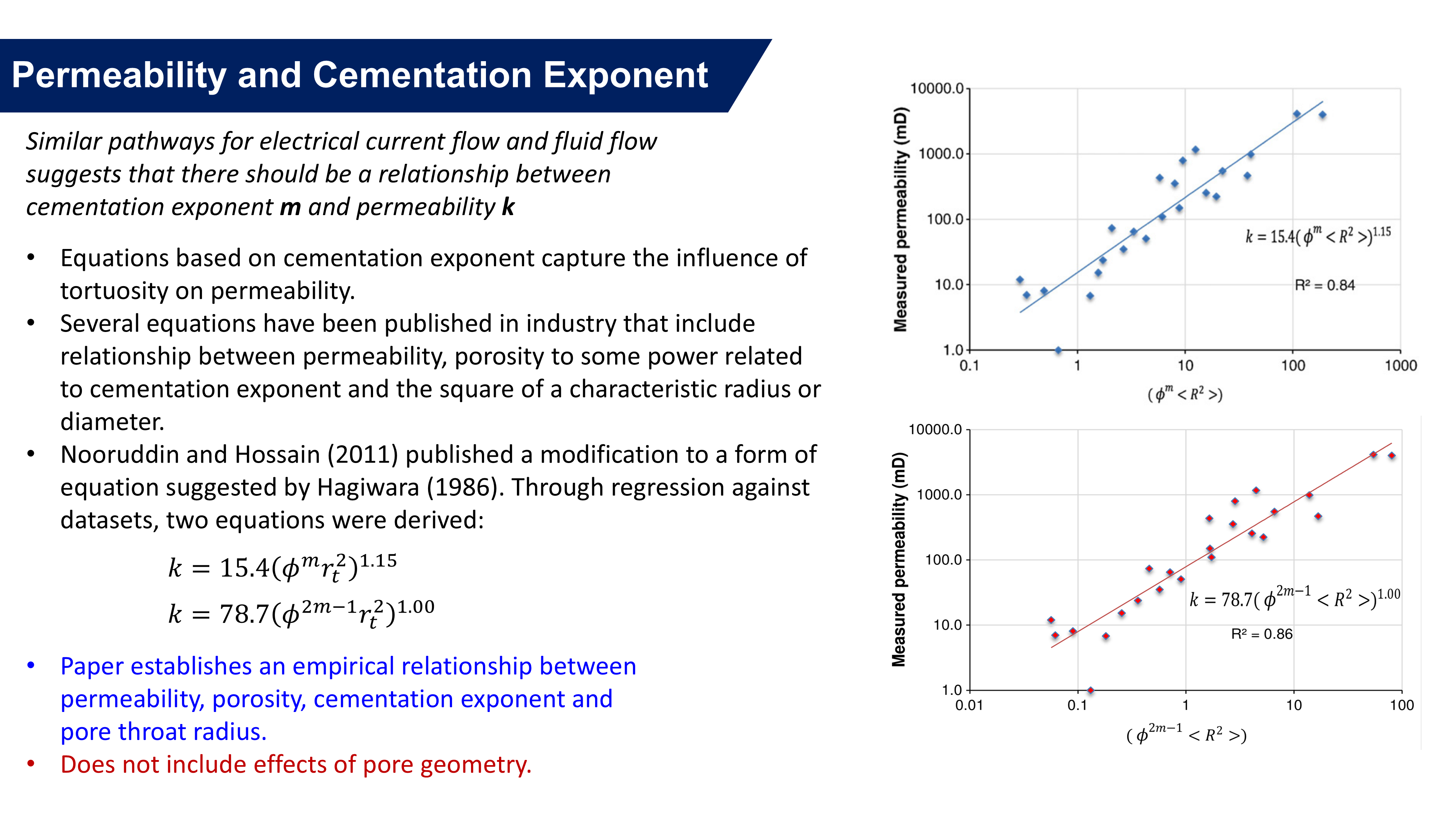
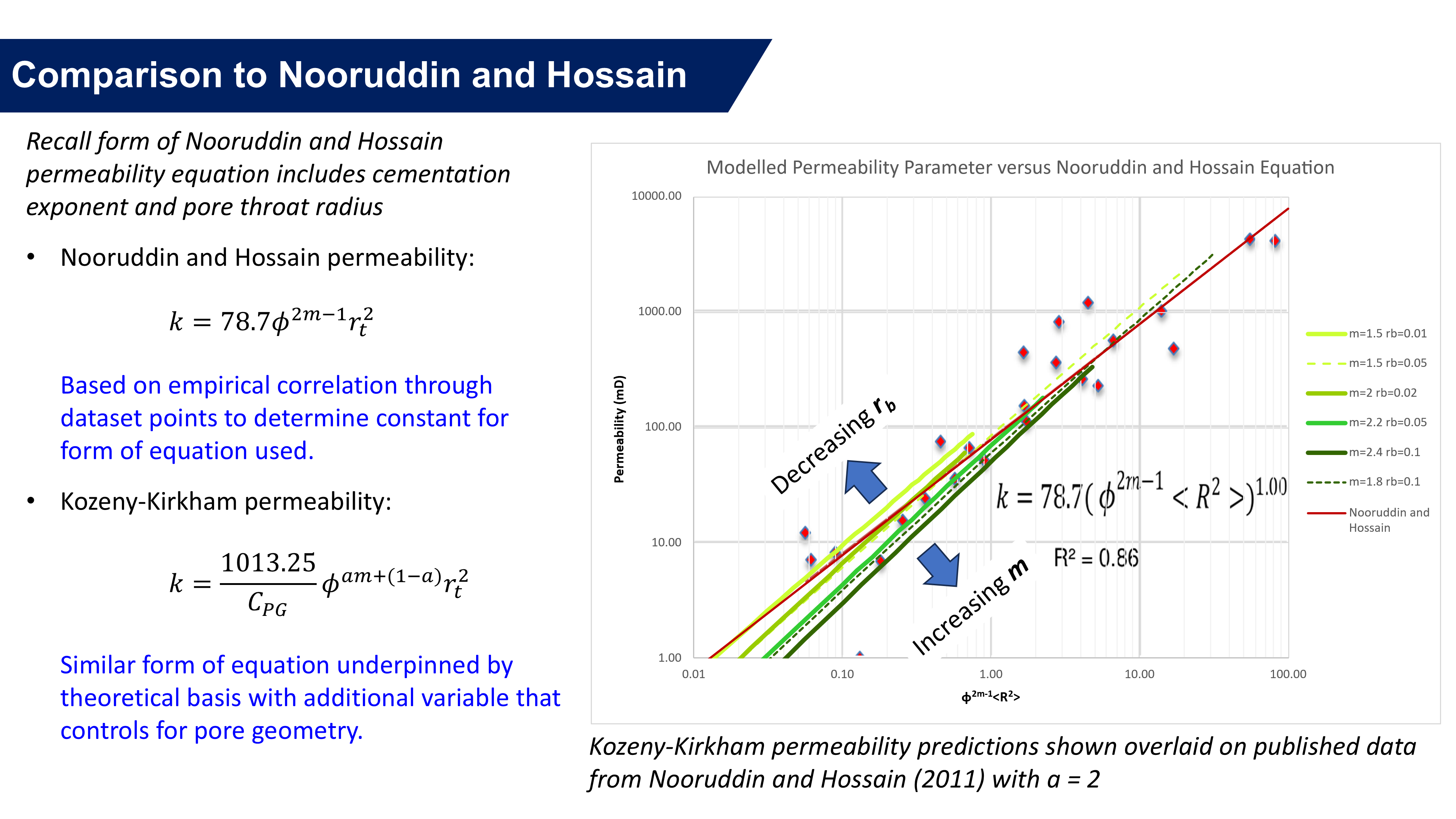
Can we predict permeability using the cementation exponent? Fortunately many researchers in the past have wondered the same thing and there are many permeability equations that incorporate cementation exponent into their form in lieu of a tortuosity term. For example there are the equations published by Nooruddin and Hossain (2011):

The form of their second equation is based on theory, and they have then regressed against this form of the equation to obtain an empirical relationship between permeability, porosity, cementation exponent and the pore throat radius. As can be seen from the charts taken from their paper on Figure 9, the fit to the dataset is not too bad.

This equation was the approach originally used by Pyrus for predicting permeability from a rock model. By first determining the cementation exponent, the Nooruddin and Hossain permeability model could be used. The equation includes three of the four proposed influences on permeability shown in Figure 3. The missing parameter is the pore geometry coefficient.

The Nooruddin and Hossain equation links together three fundamental rock properties and relates them to permeability. These properties are the porosity, tortuosity (which is captured in the cementation exponent), and the pore throat radius.

Are there other equations that link similar properties? We examine two similar equations on Figure 10. One such equation has the form proposed by Berg. It can be seen that this equation contains porosity, a characteristic length squared and a tortuosity-related term:

Where:

• φ = porosity
• d = median grain diameter (µm)
• p = sorting term P₉₀ − P₁₀ percentile deviation

Another equation is that derived by Van Baaren. It too contains porosity, a characteristic length squared and two tortuosity-related terms.

Where:

• φ = porosity
• d_d = dominant grain diameter (µm)
• m = cementation exponent
• C = sorting index 0.7 (very well sorted) to 1.0 (poorly sorted)

If we recall the fundamental properties that influence permeability shown on Figure 3, these equations essentially account for three of the four primary drivers. Tortuosity is controlled by the length of the flow paths relative to the gross length along the rock. More complex flow paths are revealed by higher cementation exponent. The pore throat radius is related to the characteristic length used in each equation. For Berg and Van Baaren, this is the average grain diameter. Small grain sizes will proportionally be associated with smaller pore throat sizes. Thus it appears that these equations all have a similar basis.

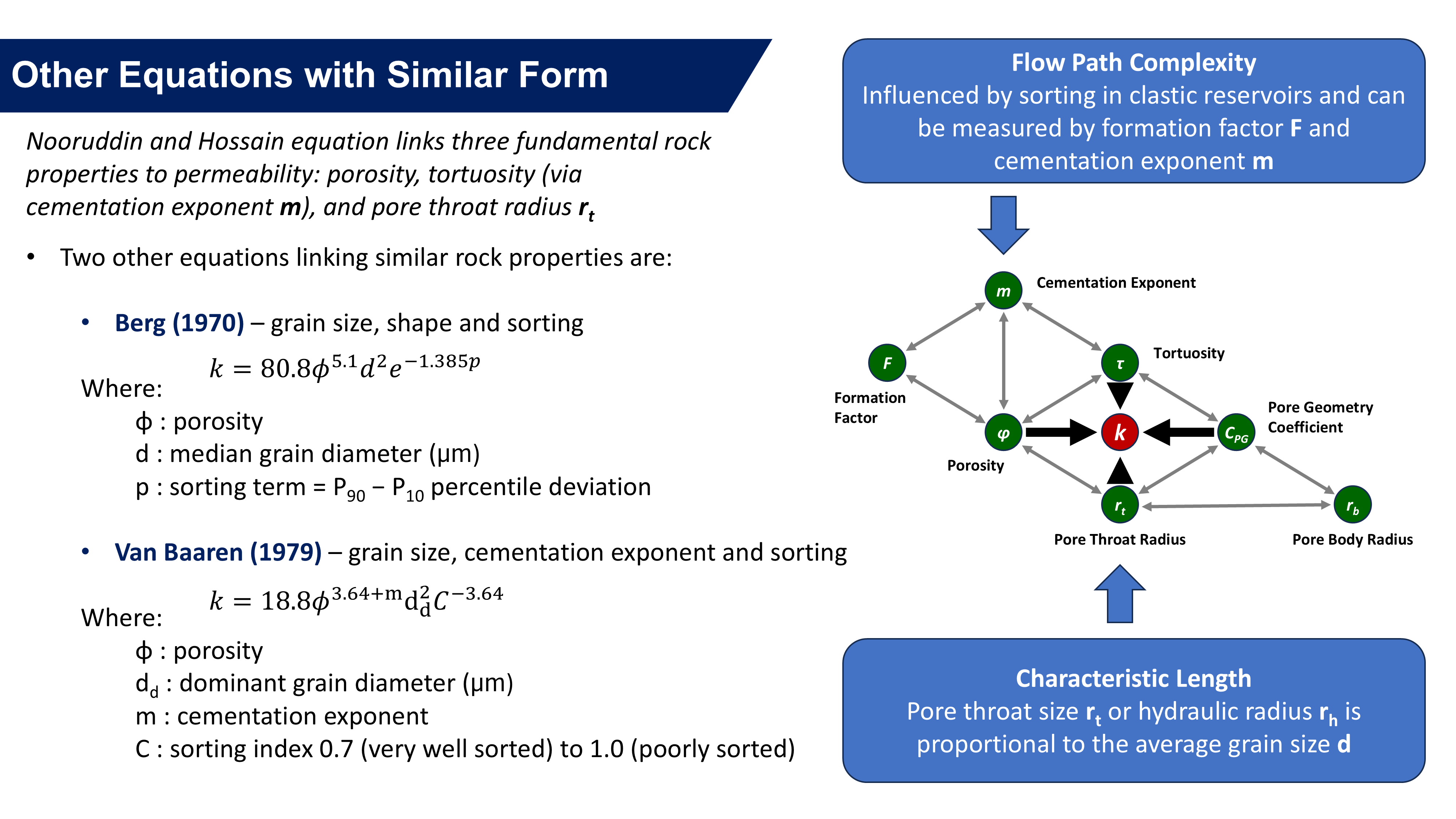
Can we do better? It is noted that these equations do not appear to take into consideration pore geometry, which we established earlier could be defined using the pore body to pore throat size ratio.

Part IV Video - Predicting Permeability with Cementation Exponent

Derive Kozeny Permeability Using Modified Pore Throat Model

To develop a more general permeability solution, let’s revisit Kozeny and attempt to re-derive the equation, but this time using a modified pore throat model which also includes the effect of tortuosity.

The Müller-Huber, Schön and Börner modified pore throat model allows a relationship between pore geometry and cementation exponent to be created. From here, the cementation exponent can be applied to various permeability equations that incorporate cementation exponent. It should also be possible to re-derive the Kozeny equation using a modified pore throat model instead of the conventional capillary tubes. The logic for pursuing this approach is that it might reveal a superior form of the Kozeny equation.

Part V Slides - Derive Kozeny Permeability Using Modified Pore Throat Model

The overall outline of the modification procedure is shown in Figure 11. The modified pore throat model used by Müller-Huber, Schön and Börner did not include the effects of tortuosity through the actual length of the tube. Our first step will be to include this term as it is important to capture tortuosity in the Kozeny form of equation.

Having set up the initial equations, a similar workflow to that used by Müller-Huber, Schön and Börner will be used. Next We will substitute in the Hagan-Poiseuille equation into the Darcy equation, and then through further substitution and rearrangement end up with an expression for permeability. Finally we will need to check that the incorporation of tortuosity has not inadvertently changed the model. By setting tortuosity to one, we should get the same model as the one that was published.

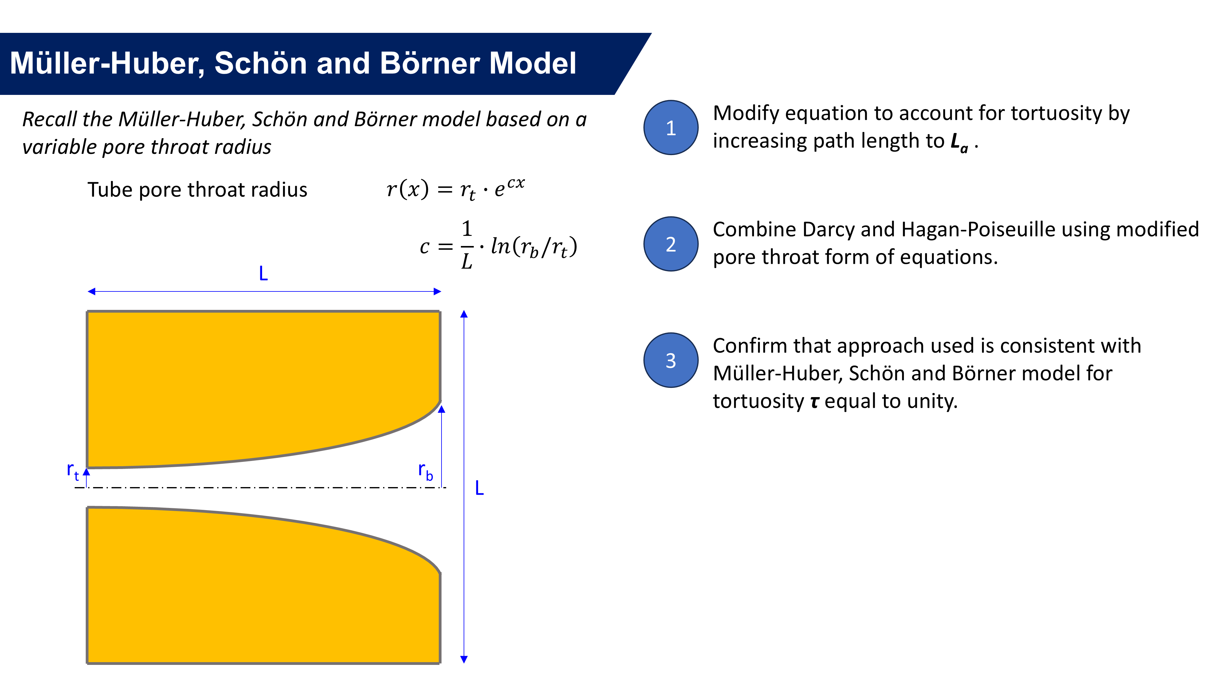
As shown in Figure 12, our modified pore throat model is simply a longer tube of length L a.

Note that the unit volume for the rock model is still L by L by L. The illustration here only relates to the path along the tube itself. Other than the use of the actual length, this is otherwise identical to Müller-Huber, Schön and Börner. However, it is the introduction of actual length that allows us to capture tortuosity in the Kozeny equation, as distinct from the variable pore body to pore throat sizes, so this is a crucial nuance.

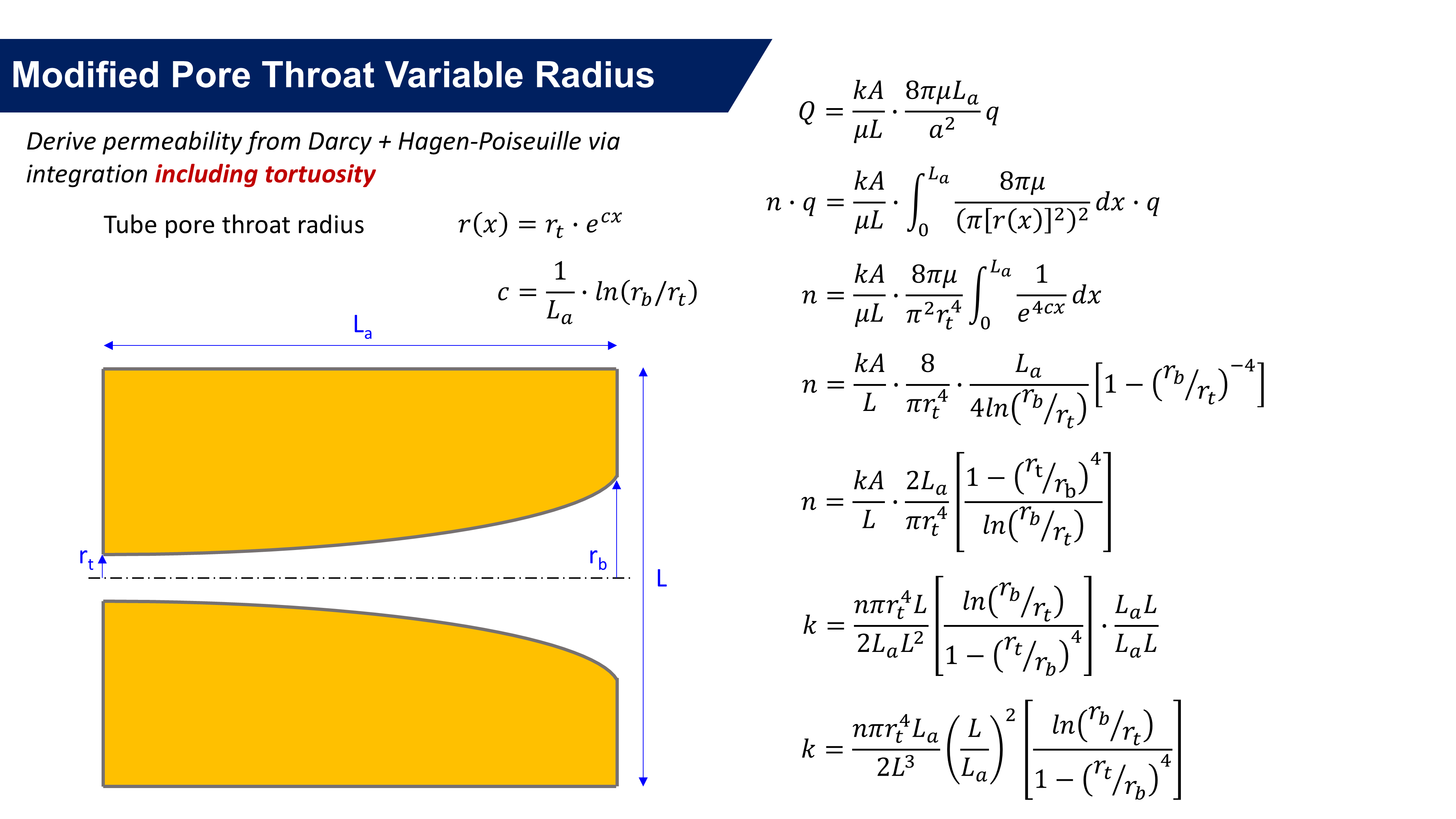
We start with substitution of Hagan-Poiseuille into Darcy and get stuck into the math … There’s a bit more integration required in comparison, and I won’t laboriously step over each line. You’ll have to take my word for it that the derivation is correct. If we skip to the last line, what we see is that we do end up with an equation for permeability which seems to incorporate tortuosity which is by definition \(\left(\frac{L_a}{L}\right)^2\).

This is encouraging as it means that we appear to be heading on the right path to replicate the Kozeny equation, but using a variable pore throat model instead of the capillary tube model.

Somehow we now need to substitute porosity into the permeability equation. This isn’t as straightforward as simply calculating the volume of a thin cylinder as with the capillary tube mode.

Instead we must integrate over the actual length to get an expression for porosity in terms of the modified pore throat model. We need to multiply permeability by some terms with identical numerators and denominators so that permeability can be expressed in terms that appear similar to other parameters. Once we have manipulated the expression, it is easy to see on Figure 13 where porosity (shown in green outline) and tortuosity (shown in blue outline) fit in.

Substitution into the equation reveals a modified Kozeny equation. As will be shown later, the term containing the pore geometry in \(\frac{r_b}{r_t}\) reduces to \(\frac{1}{8}\) as \(\frac{r_b}{r_t}\) tends to unity.

What we have defined is a more general form of the Kozeny equation for variable pore body sizes:

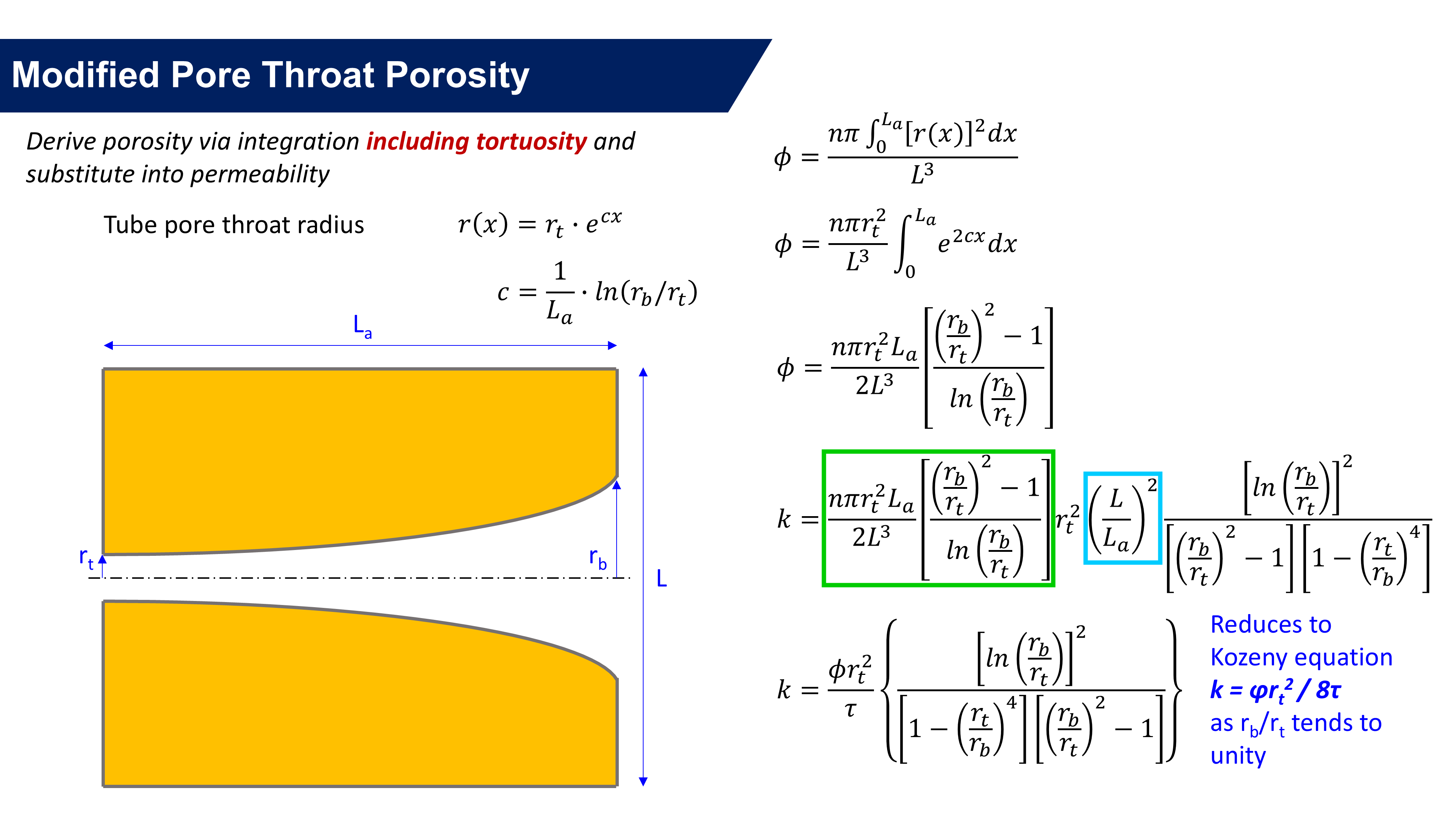
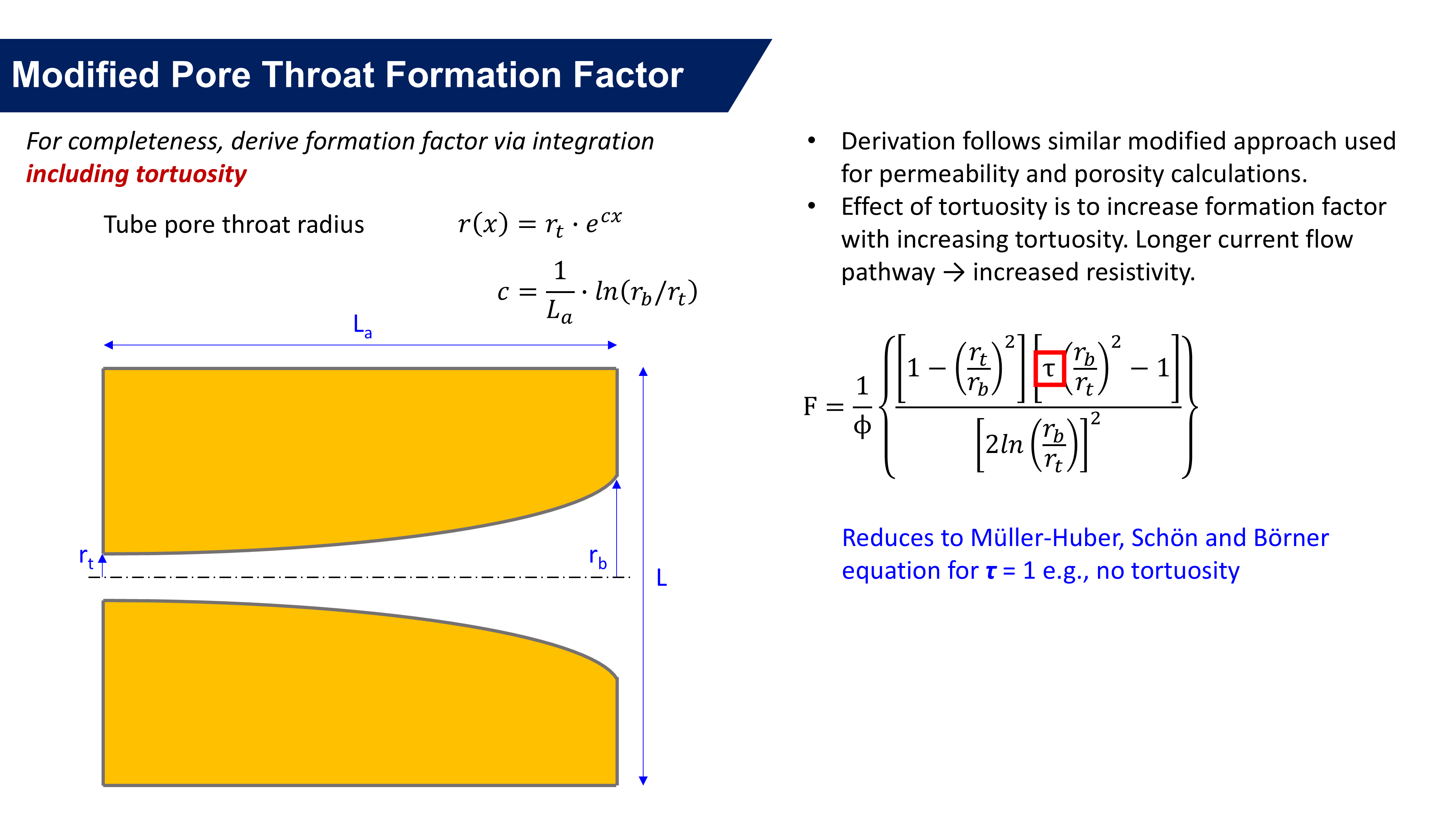
As a final check, we ensure that the addition of tortuosity has not ruined the original expression for the formation factor derived by Müller-Huber, Schön and Börner. We won’t walk through the derivations again and instead skip straight to the answer which is shown in Figure 14.

Tortuosity appears as a single additional term to the formation factor equation. The effect of this addition is to increase the formation factor if tortuosity increases. This is as expected. Furthermore, if we set τ to 1, then the equation reduces to the same form as that proposed by Müller-Huber, Schön and Börner.

This suggests that the incorporation of tortuosity into the equation has been treated correctly.

Part V Video - Derive Kozeny Permeability Using Modified Pore Throat Model

The Kozeny-Kirkham Permeability Equation

All the pieces are now in place. With the modified pore throat model we can derive a more general form of the Kozeny permeability model which I’ll refer to as the Kozeny-Kirkham model.

It is possible that someone has previously derived this form of the Kozeny equation. After all, it is not particularly obscure or complex. That said, I’ve never seen this mentioned anywhere else in the literature. To be best of my knowledge it is novel.

The Pyrus rock model is built around several relationships that allow prediction of unknown rock properties from other known values. One such relationship is the Kozeny-Kirkham permeability equation which allows prediction of permeability from known porosity and a geological description of the rock fabric. As we will show, it is a very general (albeit theoretical) form for a permeability equation.

Part VI Slides - The Kozeny-Kirkham Permeability Equation

Let’s derive the general form of the Kozeny-Kirkham permeability equation as shown in Figure 15.

First we need to express our modified Kozeny equation a little more simply. We’ll introduce a variable C_PG which we’ll refer to as the pore geometry coefficient. It is given by this expression involving the pore body to throat ratio.

Now we follow a similar approach to Nooruddin and Hossain. We combine the equation for tortuosity by Wyllie and Rose with the simplified Archie equation. The tortuosity exponent a is given by Wyllie and Rose (1950) as 2, but other authors have such as Winsauer, Shearin, Masson and Williams (1952) have found that this value applies to unconsolidated sands but can decrease below 2 as tortuosity increases. They found that a value of 1.67 was a good match to core plug measurements.

Substitution of the Archie formation factor into the tortuosity equation gives an expression for tortuosity in terms of porosity and cementation exponent. Now we can substitute this new tortuosity term back into our permeability equation. This has the advantage that the permeability expression is now expressed in terms of cementation exponent rather than tortuosity. This is arguably a more familiar parameter.

Finally we have to convert to oilfield units. Our pore throat radius is typically given in units of micrometres. To convert to millidarcy we must multiply by 1013.25. This gives the final form of the Kozeny-Kirkham permeability equation:

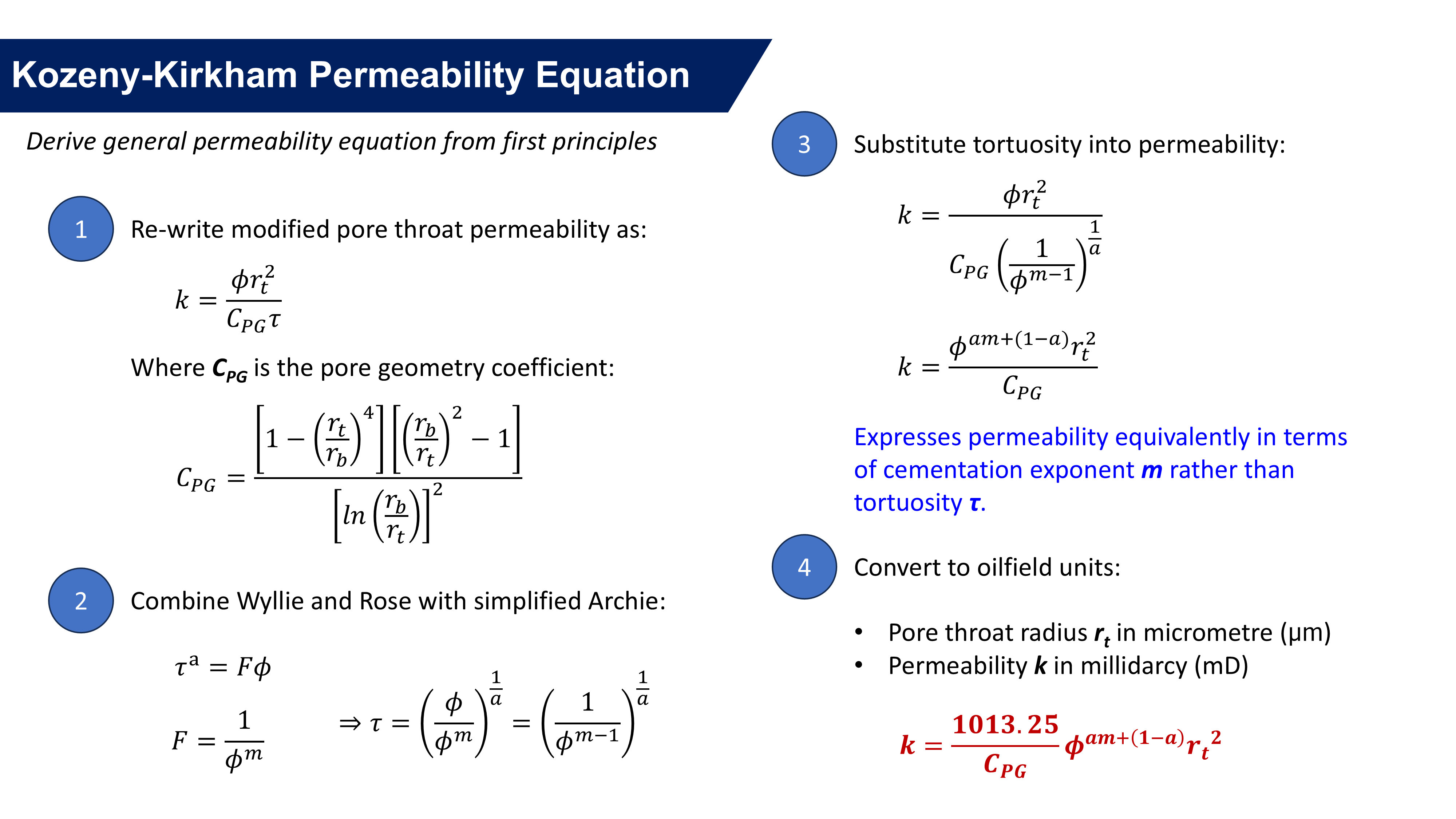
If the form of the equation looks familiar, it is because it is. Recall the Nooruddin and Hossain equation. This is based on an empirical correlation to fit a theoretical form of an equation.

The Kozeny-Kirkham equation is based on a similar theoretical form, but rather than using an empirical correlation to fit a dataset, the constant in the Nooruddin and Hossain equation is instead represented by a term that captures the effects of pore geometry.

A comparison of the two equations is shown in Figure 16. On the right we can see the datapoints used by Nooruddin and Hossain to obtain the slope of 78.7. If we superimpose the results for the Kozeny-Kirkham equation on top of this plot, it is very quickly seen that the trends do not violate any of the data.

Lines have been plotted for a range of different cementation exponent (from 1.5 to 2.4) and a range of different pore body radii (from 10 microns to 100 microns). In addition dashed lines are shown so that the effect can be observed of just changing pore body radius whilst keeping cementation exponent constant, or vice versa, changing cementation exponent whilst keeping pore body radius constant.

The effect is that the permeability prediction is moved by changing r_b and / or cementation exponent. By including the pore body radius it appears that the variability in the dataset could be better explained by the Kozeny-Kirkham permeability equation.

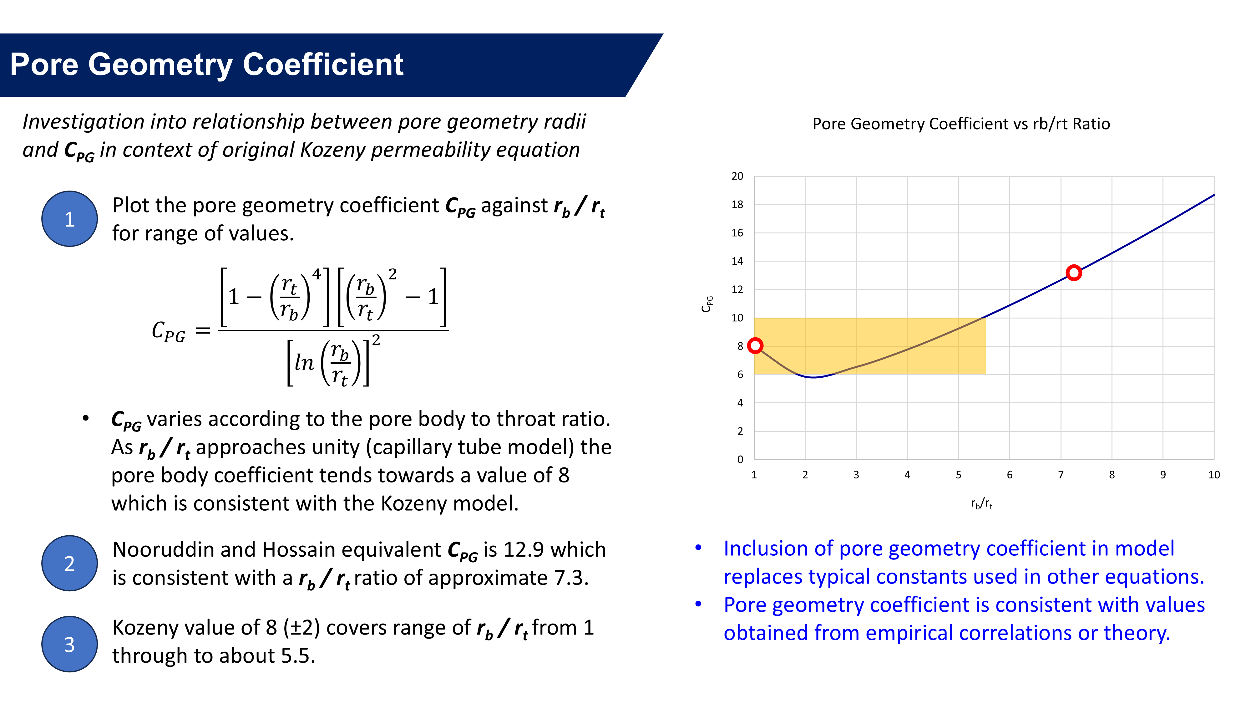
The inclusion of the pore geometry coefficient gives meaning to the constants in the Kozeny and Nooruddin and Hossain equations.

We can plot the variation in pore geometry coefficient against the pore body to throat ratio as shown in Figure 17. At a ratio of 1, where the pore body and pore throat are identical in size, the pore geometry coefficient tends towards 8, which is the same as that in the Kozeny equation. Similarly, we can plot the Nooruddin and Hossain equivalent pore geometry coefficient, which is 12.9. This is consistent with a pore body to throat ratio of about 7.3.

Sandstones and carbonates can typically have a pore body to throat ratio of five or more, so this appears at first glance to be a reasonable value to use as an average. This is not too surprising given that the value is obtained from an empirical regression.

We can also look at the range of pore body to throat ratio to which the Kozeny equation value of 8 applies. Crudely, it would be relevant up to values of 5.5. Since this is at the lower end of what is typically observed in real rocks, it indicates why the simplified capillary tube model that is the basis of the Kozeny equation means it is not of practical use.

In summary, the pore geometry coefficient replaces constants used in several other equations and explains the physical meaning of those constants.

Part VI Video - The Kozeny-Kirkham Permeability Equation

Predicting Permeability for Different Reservoir Rock Types

The Pyrus rock model based on the Kozeny-Kirkham permeability equation shows promise for being a generalised equation that can predict properties for several different rock types. Testing the versatility of the equation and its applicability to different reservoir rock types will be looked at in this last part of this post.

The new Kozeny-Kirkham permeability equation that is being proposed has a sound theoretical foundation. This is irrelevant if it cannot be usefully applied to real world reservoir rock types. To examine the relevance of this equation, the use of this equation in the context of a range of sandstones and carbonates is shown.

Part VII Slides - Predicting Permeability for Different Reservoir Rock Types

Our first step is to check how the Kozeny-Kirkham equation compares to other accepted equations for specific rock types.

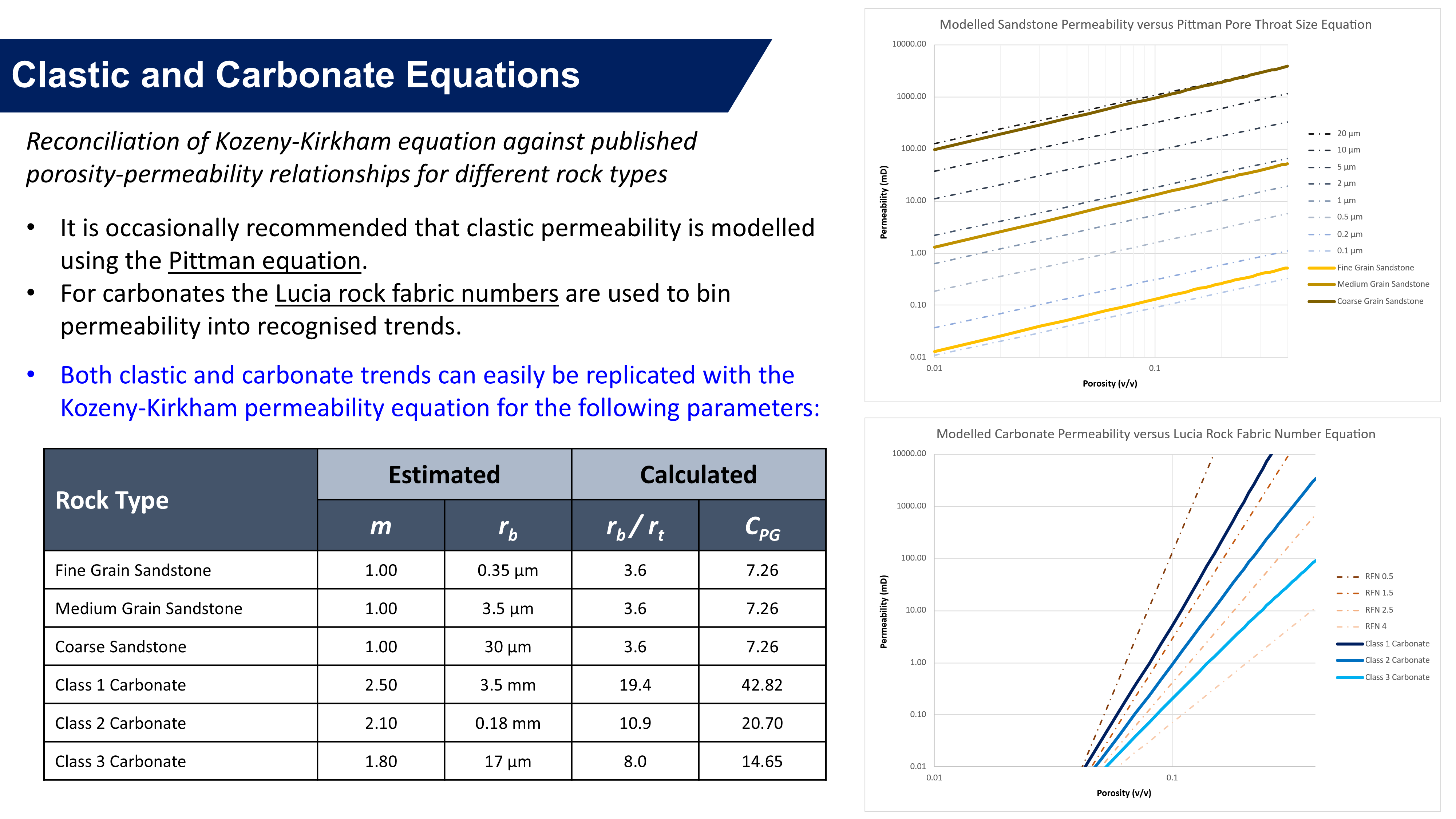
For sandstones it is often recommended to use the Pittman equation, where the permeability varies in accordance with the pore throat radius.

For carbonates, Jennings and Lucia (2003) have plotted porosity / permeability trends based on the rock fabric number.

Whilst these equations are not gospel, it is essential that the Kozeny-Kirkham equation is able to replicate results obtained by using them. It can be seen in Figure 18 that both sandstone and carbonate relationships can be modelled using the Kozeny-Kirkham equation.

The estimated values shown in the table on Figure 18 are parameters that are estimated. From these estimated values, \(\frac{r_b}{r_t}\) and hence r_t can be calculated, plus the pore geometry coefficient. To estimate our cementation exponent and pore body radius, nothing more sophisticated than a trial and error approach was used to obtain a rough match to the relevant equation.

It is interesting to note that the Pittman equation implies a cementation exponent of 1. This is the capillary tube model. Also the pore geometry coefficient is close to 8, meaning that this is similar to the Kozeny equation with an assumption of non-tortuous capillary tubes.

The carbonate trends are achieved with estimates of cementation exponent and pore body radius that are in line with expected values. For many carbonates, a value of 2 is recommended for the cementation exponent, although it is recognised that vuggy carbonates (which have lower rock fabric numbers) can have higher cementation exponents.

The matches obtained here suggest that the use of a fixed value of 2 for carbonates is not advisable, since the true value varies depending on the rock fabric.

The generalised Kozeny-Kirkham permeability equation appears to be versatile enough to cope with different reservoir rock types.

We are getting ahead of ourselves though, as the previous example calculated values for pore throat radius and pore geometry coefficient, without any explanation as to how this was done. Let’s step back a little and work through an example workflow for the recommended approach to using the Kozeny-Kirkham equation.

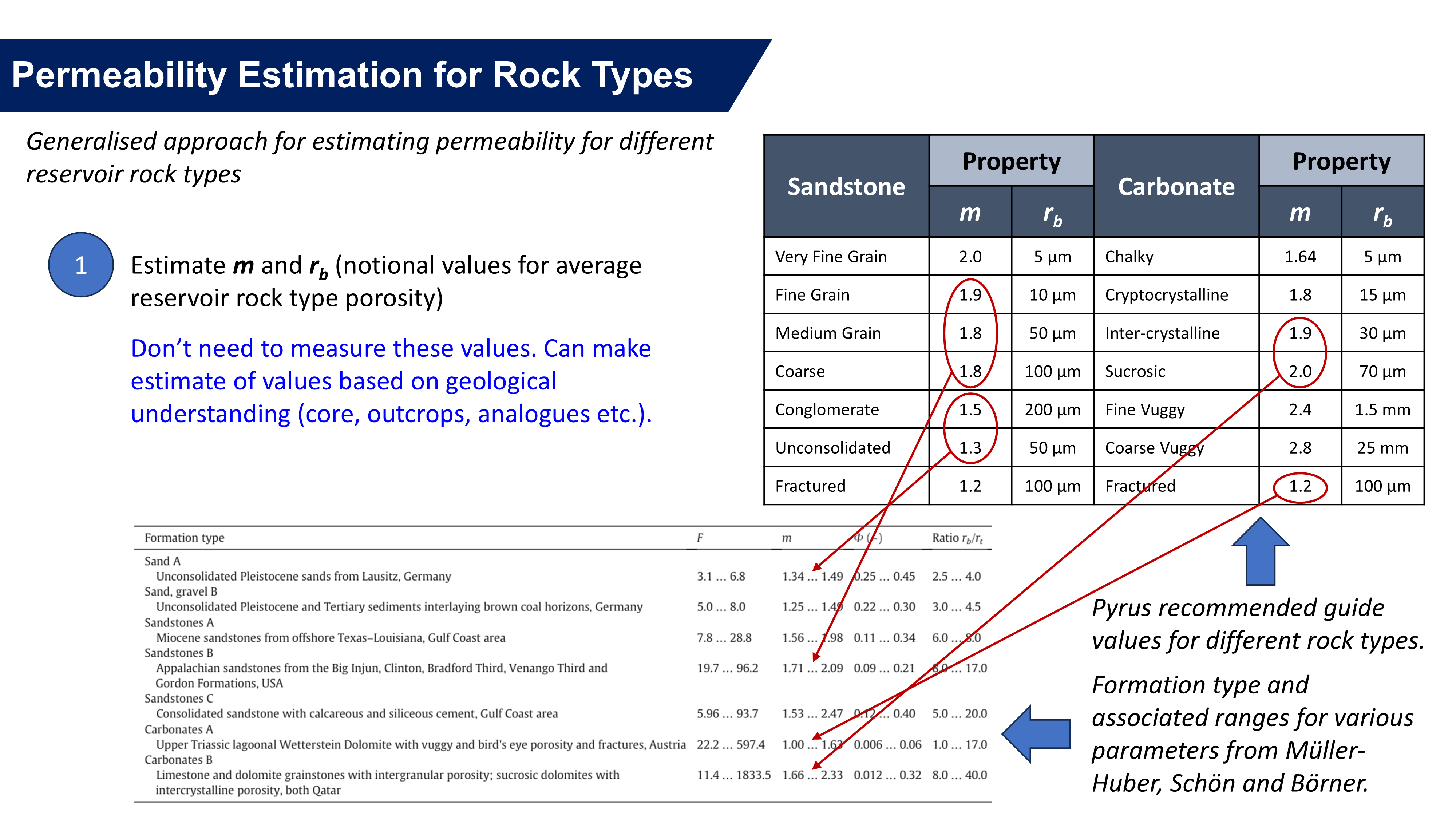
Remember, the intention with Pyrus is to be able to generate estimated, yet high quality, relationships for data where none other exists. Our first step is to estimate the cementation exponent and the pore body radius. These two parameters are intentionally chosen because a reasonable guess as to their values can be made by consideration of the geological description of the rock alone.

Let’s illustrate by example in Figure 19. Recommended values for different types of rock type are shown. It can be seen that there are variations in these properties that vary as the type of rock changes. Remember it isn’t necessary to get an exact value (if such a thing even exists, given the variability of real rock). Rather a “near enough is good enough” value can be used. For the moment I’m just going to state these recommended values. A more rigorous approach that ties these values to other measurable rock properties will be explained later.

The Müller-Huber, Schön and Börner paper that introduced the modified pore throat approach includes ranges for cementation exponent and pore body to throat ratios. It can be seen that the recommended values for cementation exponent fall within these ranges. Incidentally, the pore body to throat ratios on the previous slide are also in line with these ranges.

We have a starting point of cementation exponent and pore body radius. From these values we need to get pore throat radius and the pore geometry coefficient. We assume that porosity is known!

The first step, shown in Figure 20, is to calculate the body to throat relationship. This is a rearrangement of an earlier derived equation. The trick now is to invert this to get the pore body to throat ratio. As you can see the equation is reasonably involved.

To simplify we assume tortuosity is one and then use a regression through pre-computed values for \(\frac{r_b}{r_t}\) against R_BT. We need to use a second linear regression at large values of R_BT as the polynomial regression is not well behaved at extreme values.

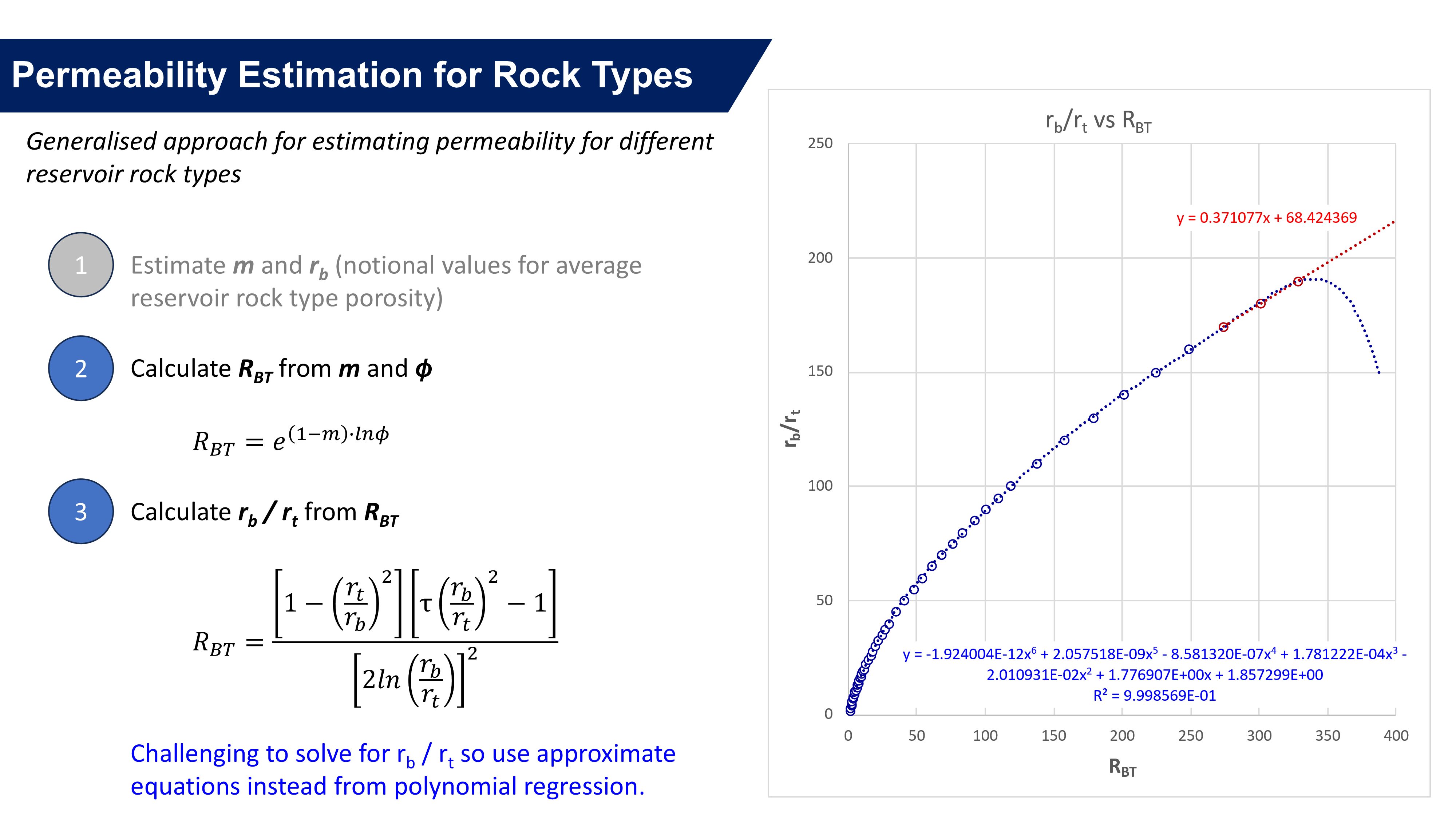
At this point we have the key to calculate our missing parameters which are the pore throat radius and the pore geometry coefficient. These can be calculated directly from the pore body to throat ratio.

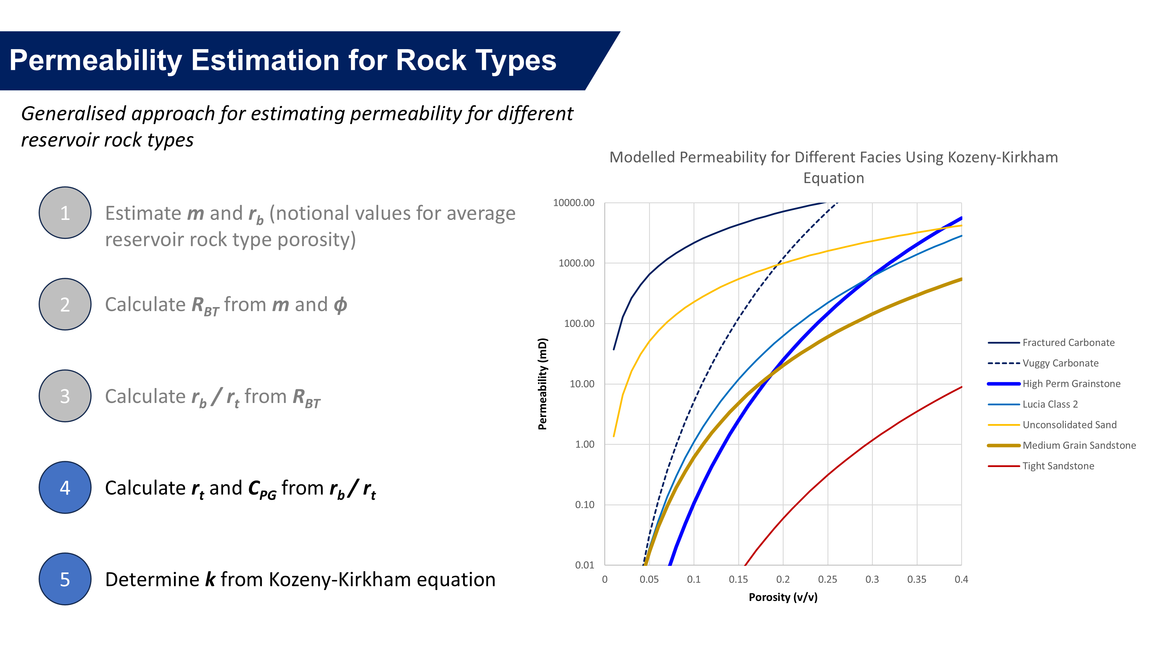
We now have all the parameters needed for the Kozeny-Kirkham permeability equation. Let’s calculate a few different rock types using this approach and plot them as shown in Figure 21.

It can be seen that this equation allows prediction of permeability across several different orders of magnitude for any given porosity. As such I consider this to be a very versatile and useful technique applied within Pyrus.

Part VII Video - Predicting Permeability for Different Reservoir Rock Types

Next Steps

This long blog post introduces the theory behind the Kozeny-Kirkham equation that is applied in the Pyrus rock model. What is not shown is how to estimate the cementation exponent and pore throat radius for different rock types, such as sandstone and carbonate. A method to estimate these parameters from grain size and sorting (in the case of sandstones), and rock fabric number and dolomitisation (in the case of carbonates) has been devised in Pyrus and will form the topic of another blog post(s).

Another post will cover comparison of the Kozeny-Kirkham permeability equation versus other popular equations, with testing against published porosity-permeability datasets.

References

• Archie, G. E. 1942. The Electrical Resistivity Log as an Aid in Determining Some Reservoir Characteristics. J Pet Technol 146 (1): 54-62. SPE-942054-G. https://doi.org/10.2118/942054-G
• Berg, R. R. 1970. Method for Determining Permeability From Reservoir Rock Properties. In Transactions of the Gulf Coast Association of Geological Societies, Vol. 20, 303-317. Tulsa, Oklahoma: American Association of Petroleum Geologists.
• Hagiwara, T. 1986. Archie’s “m” for Permeability. The Log Analyst 27 (1): 39-42.
• Jennings, J. W. Jr. and Lucia, F. J. 2003. Predicting Permeability From Well Logs in Carbonates With a Link to Geology for Interwell Permeability Mapping. SPE Res Eval & Eng 6 (4): 215-225. SPE-84942-PA. https://doi.org/10.2118/84942-PA.
• Müller-Huber, E., Schön, J., and Börner, F. 2015. The Effect of a Variable Pore Radius on Formation Resistivity Factor. Journal of Applied Geophysics 116 (2015): 173-179. https://doi.org/10.1016/j.jappgeo.2015.03.011.
• Nooruddin, H. A. and Hossain, M. E. 2011. Modified Kozeny-Carmen Correlation for Enhanced Hydraulic Flow Unit Characterization. Journal of Pet. Sci. Eng. 80 (1): 107-115. https://doi.org/10.1016/j.petrol.2011.11.003
• Van Baaren, J. P. 1979. Quick-Look Permeability Estimates Using Sidewall Samples and Porosity Logs. In Transactions of the 6th Annual European Logging Symposium. Society of Professional Well Log Analysts.
• Winsauer, W. O., Shearin, H. M. Jr., Masson, P. H., and Williams, M. 1952. Resistivity of Brine-Saturated Sands in Relation to Pore Geometry. AAPG Bulletin 36 (2): 253-277. https://doi.org/10.1306/3D9343F4-16B1-11D7-8645000102C1865D.
• Wyllie, M. R. J. and Rose, W. D. 1950. Some Theoretical Considerations Related to the Quantitative Evaluation of the Physical Characteristics of Reservoir Rock from Electrical Log Data. J Pet Technol 2 (4): 105-118. SPE-950105-G. https://doi.org/10.2118/950105-G.