To analytically assess the production rate obtained from a well requires both an understanding of the inflow performance relationship (IPR) that governs from a reservoir into a wellbore for a given pressure drawdown, and the vertical lift performance (VLP) of fluids that can flow up the wellbore tubing for a given downhole and tubing head pressure differential. The combination of IPR and VLP is known as “nodal analysis” as it seeks to identify the pressure at the bottom hole node where the IPR and VLP flow rates match.
Generating a VLP curve that describes the variation in bottom hole pressure required to achieve different flow rates in a well is non-trivial. It can be done by hand, or more conveniently in a simple spreadsheet, but this approach often relies on fluid property correlations and simplifying assumptions, which can add inaccuracies into the results obtained. From the very early days of computing, this was a problem that was perhaps better tackled via a dedicated progam. The early days of PIPESIM is a fascinating look into the origins of one commercial industry solution to this problem. Naturally, writing your own pipe flow program is a challenge that I couldn’t resist.
How should one approach this problem? Flow of multiphase fluids in pipe is a problem encountered in many different fields, not just oil and gas. There is a wealth of research and literature on the subject. For better or worse, within the oil industry what I will describe as a “classical” approach has emerged. The classical approach is largely empirical in nature, and in fairness, if it works there shouldn’t be a problem. The issue is that the oil industry appears to have ventured down a path of ever increasing complexity, where models have become more sophisticated, and the software costs have risen in tandem. In the process, the tools have become black boxes. A colleague related a story to me where an E&P contractor had run into an issue with “vapour lock” predicted by one of the commercial software tools, although there was no physical expectation of that occuring in the scenario being modelled. Apparently this caused huge issues because no-one was able to challenge the software result, and their team had to resort to solving the problem in a different way, and at higher cost.
Recently, I came across a PhD dissertation by Dr. Anand Nagoo which flipped this whole approach on its head. Approaching the problem from a “fundamental” first principles approach, Nagoo proposes a simpler analytical method, which is then tested against a large database of published experimental and real-world data. It appears that in many cases this outperforms the available commercial solutions. Perhaps this shouldn’t be too surprising: in reservoir simulation a simple material balance model can sometimes give better insight and results than a highly detailed multi-cell compositional model. Garbage-in garbage-out. As Dr. Nagoo notes in the conclusion to his dissertation:
“simple, suitably-averaged analytical models can yield an improved understanding and significantly better accuracy than that obtained with extremely complex, tunable models.” (Nagoo, 2013)
Simpler. Faster. More accurate. The lure of this fundamental approach is undeniable. The question is, “how does it compare”?
This blog post sets out a comparison between the two different approaches that have been implemented in Pyrus.
The Hydrocarbon Multiphase Pipe Flow Problem
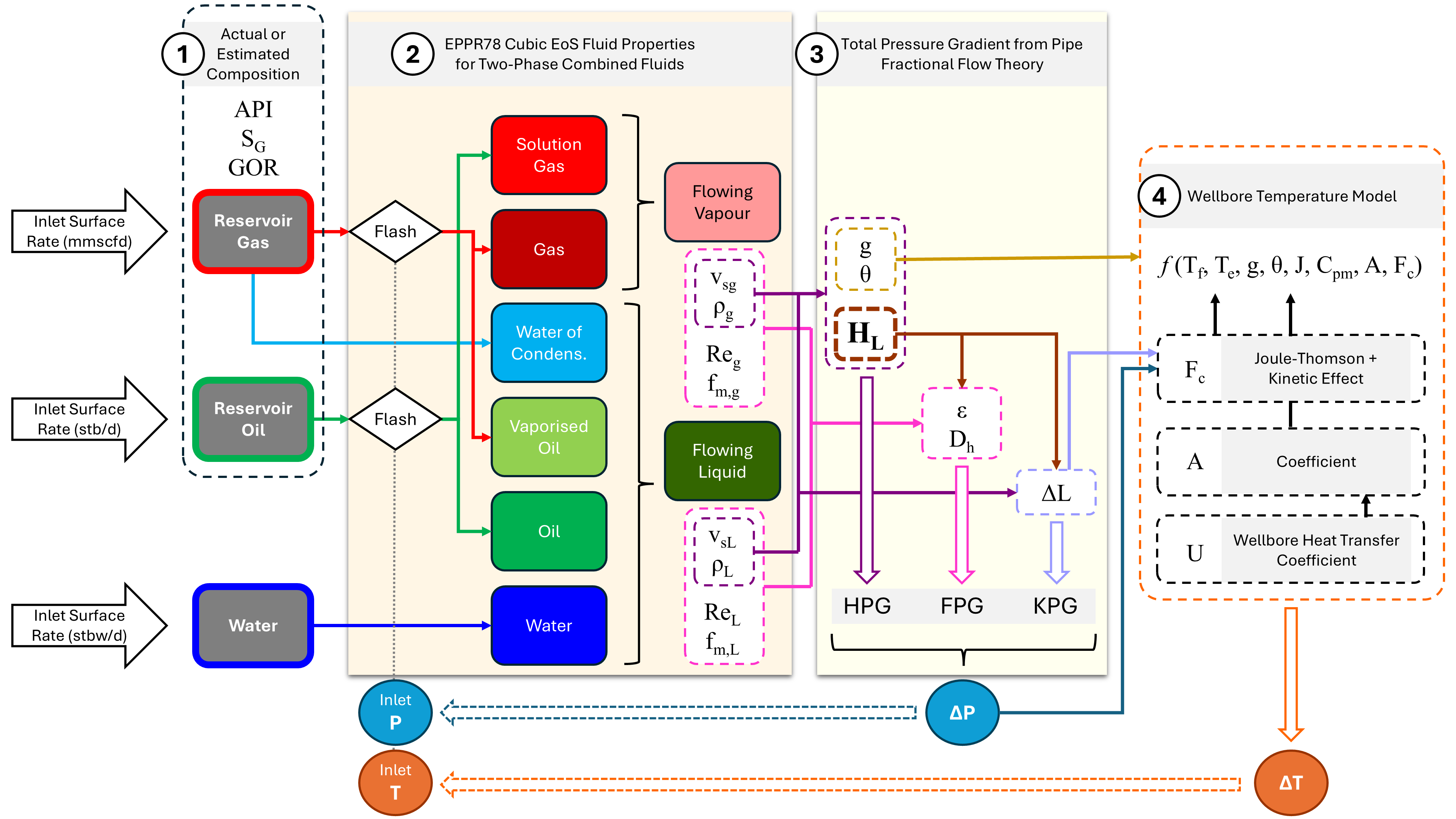
As if equation of state modelling wasn’t hard enough already! What happens when we place our reservoir fluid into a well and produce it from the subsurface to the surface via tubing? There are a multitude of simultaneous phenomena that are continuously evolving and must be considered in any simulation/model of hydrocarbon flow in a pipe. It’s all related to heat and mass balance, whereby the mass and energy (kinetic, potential and thermal) must be conserved, whilst simultaneously affecting the PVT (pressure, volume and temperature) properties of the fluid flowing in the pipe.
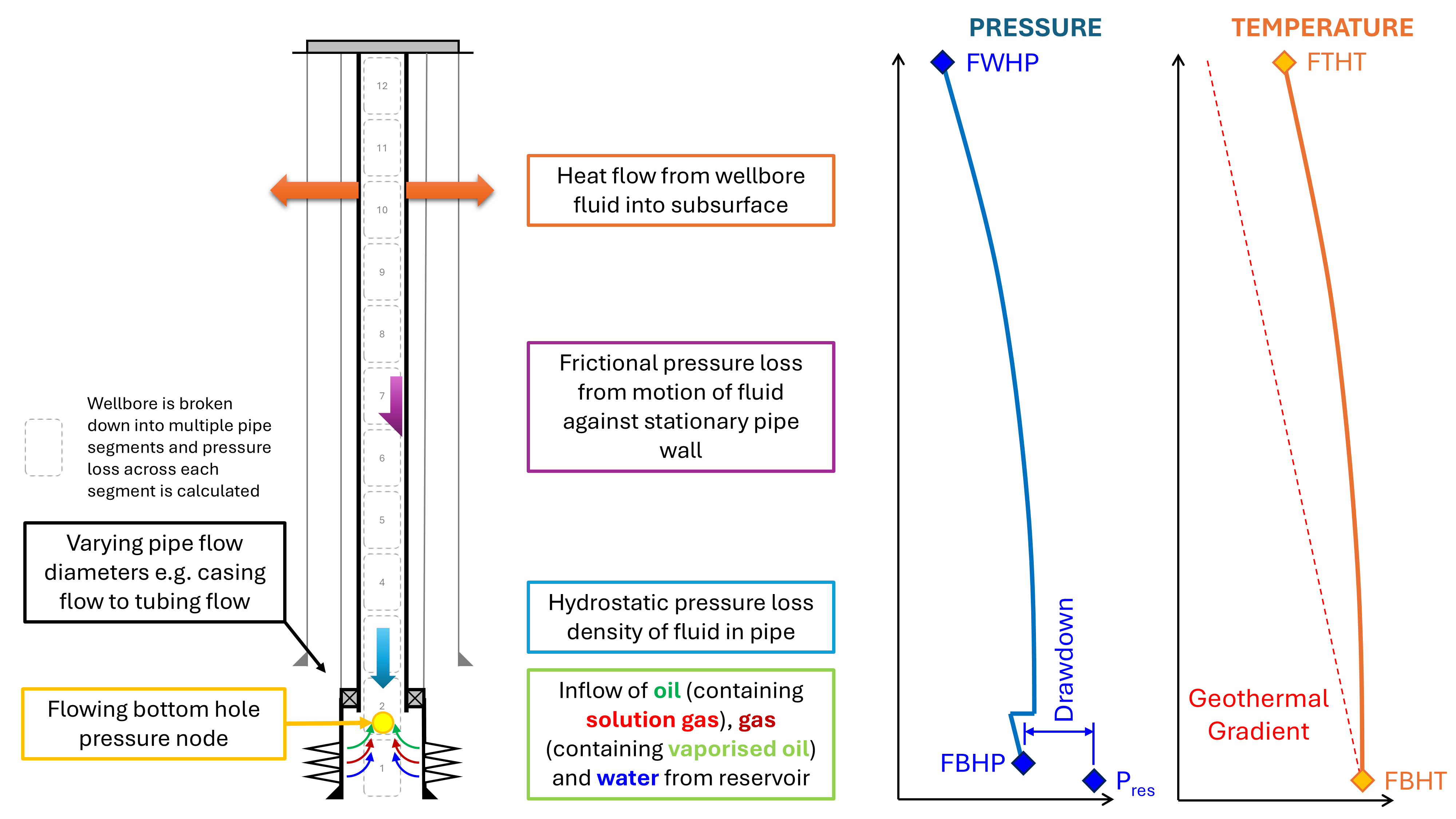
Initially the fluid is found at the reservoir pressure and temperature. The reservoir inflow performance relationship will determine the flow rate, and thus volume, of reservoir fluid that will flow for a given drawdown (pressure differential) between the reservoir pressure and the flowing bottom hole pressure (FBHP). At the inlet point of the tubing there exists an inlet pressure (which will be close to the FBHP if the tubing is close to the perforations depth) and an associated flowing bottom hole temperature (FBHT). The FBHP is less than the reservoir pressure. For an oil the FBHT should be similar to the reservoir temperature, but for a gas that has undergone significant expansion, this may be cooler due to the Joule-Thomson effect.
If the FBHP is sufficiently high to overcome the opposing forces that prevent or restrict flow of fluid in the pipe, then the hydrocarbons will begin to flow.
In a steady state condition, there are three forces to consider:
- Hydrostatic force: being the action of gravity acting on the mass of the fluid itself.
- Frictional force: being the shear force exerted on the fluid by the stationary pipe wall.
- Kinetic force: resulting from accelerative or decelerative conditions.
In addition, the fluid stores heat. This heat is convected along the wellbore, but the presence of a (generally cooler) geothermal gradient in the subsurface means that some of this heat is continuously conducted out of the well. The radial heat transfer out of the wellbore becomes more significant as hotter fluid from deep in the subsurface reaches a cooler environment near to the surface.
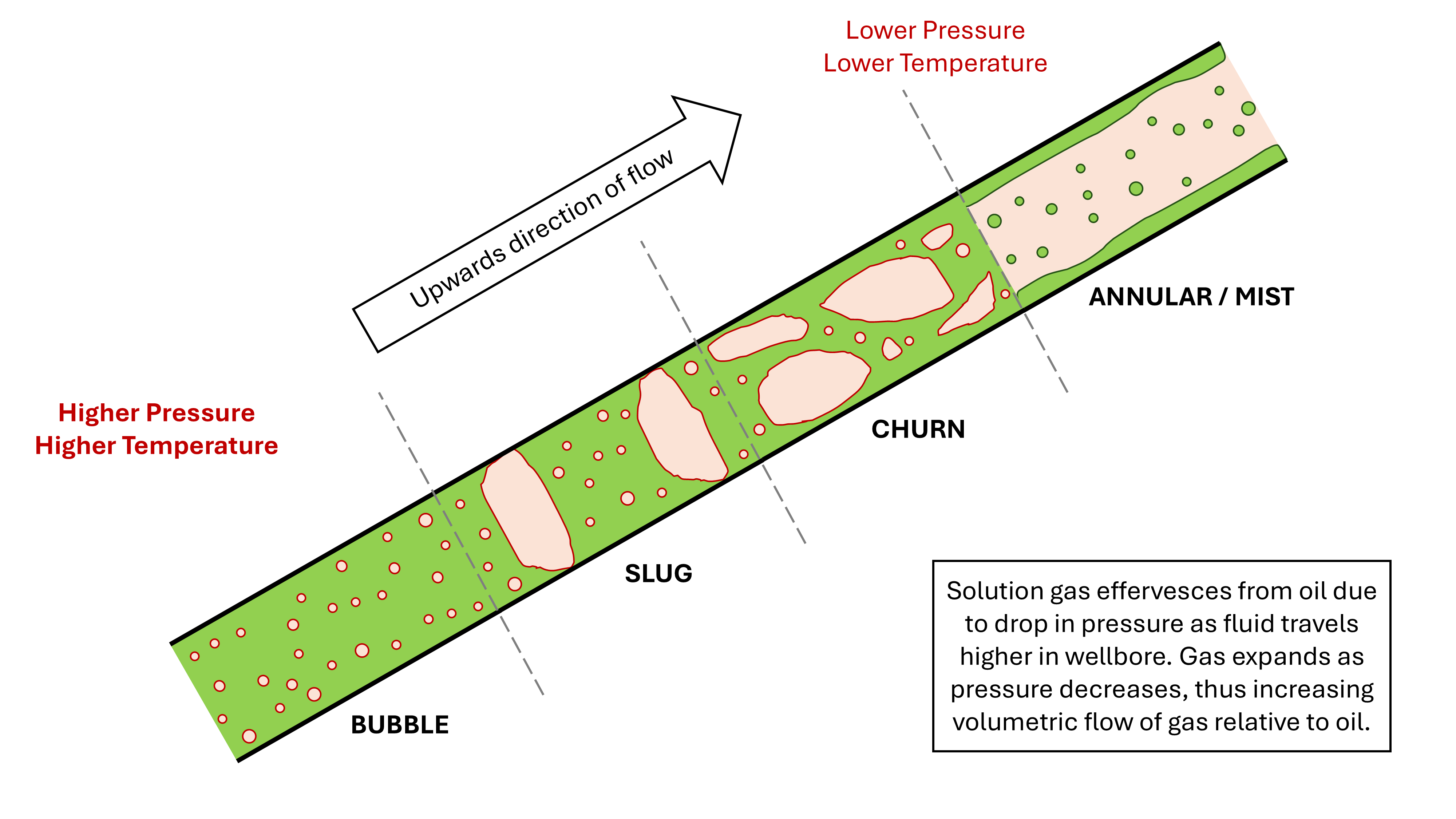
If the fluid in question is largely incompressible and exists in a continuous single phase condition at all temperature and pressure conditions in the wellbore, then this can relatively straightforward. Hydrocarbons are “way too cool” to turn up at that party. The pressure and temperature will vary along the wellbore, meaning that the fluid may enter the two-phase region. Solution gas may evolve from an oil below bubble point, or vaporised oil may condense from a gas below the dew point. This gives rise to a multiphase flow environment in the wellbore, and depending on the relative volume of liquid and vapour phases. Because of buoyancy and other effects, each phase may have a different flowing velocity, such as the phenomenon of gas bubbles rising up through a dominant oil phase in vertical pipe, leading to faster gas velocity in comparison to liquid velocity. The difference between the phase velocities influences the hydrostatic, frictional and kinetic forces.
At the wellhead, the outlet conditions from the wellbore are known. These are the flowing well head pressure (FWHP) and the flowing tubing head temperature (FTHT). If the simulation is sufficiently accurate, the downhole FBHP can be predicted by matching the FWHP predicted by the simulation to the actual measured value. In theory, if the multiphase pipe flow problem is sufficiently well solved, it is possible to infer downhole conditions from surface measurements alone.
The result is that there is an interplay between the multiphase energy conservation equations (heat and mass balances) that arise from the flow of fluid in the pipe, and the equation of state that governs the nature (phase, volume and properties) of each of the phases present in the pipe.
All this for something as apparently simple as flow of a fluid in a stationary pipe!
Approaches to Solving the Multiphase Pipe Flow Problem
There are two approaches that have been used to solve the multiphase pipe flow problem in Pyrus. As noted earlier, I have termed these the “classical” approach that uses the oil industry generally accepted principles and a more recent “fundamental” approach based on pipe fractional flow theory. I describe and compare the approaches here, not necessarily to promote or dismiss either approach, but rather to help explain the steps involved, in case others might want to write their own multiphase flow simulator as I have done.
Classical Approach
The classical approach taken to solving multiphase flow is driven by empirical correlations to determine the volume fraction of a given segment of pipe that is occupied by each phase, and its respective velocity. Further complicating matters is that with two-phase flow it is possible that velocities of the vapour and liquid phases are different. A consequence of this is that the liquid and gas volume fractions at any given cross-sectional area of the pipe will not be the same as the ratio of phase volumetric flow rate to the total volumetric flow rate.
Conventionally the determination of this difference is driven by first predicting the flow pattern map, and from the flow pattern map the slip velocity (difference between the vapour and liquid velocities) is calculated. In turn, the liquid volume fraction can be obtained from the slip velocity. Note that this approach relies on any assumptions used for the unknown flow pattern, and whilst there are only a few different recognised flow patterns, the boundaries between each of these patterns is somewhat subjective and varies between researchers.
For the common two-phase scenario with vapour and liquid phases, the liquid volume fraction is often referred to as the liquid holdup with the symbol \(H_{L}\) in the classical approach. Liquid holdup is defined simply as:
\[H_{L} = \frac{V_{L}}{V}\]Where:
- \(V_{j}\) = volume of phase-j in pipe segment with j = liquid (L) or gas (g)
- \(V\) = volume of pipe segment
Classical Hydrostatic Gradient
Assuming the liquid holdup is known, and the density of each fluid is known, it is straightforward to calculate the hydrostatic gradient:
\[\rho_{mix} = \rho_{L} \cdot H_{L} + \rho_{g} \cdot (1 - H_{L})\]Where:
- \(\rho_{j}\) = phase-j density with j = liquid (L) or gas (g)
Once the fluid density is known the hydrostatic pressure gradient is calculated as:
\[HPG = \rho_{mix} \cdot g \cdot cos(\theta)\]Where:
- \(HPG\) = hydrostatic pressure gradient (psi/ft)
- \(g\) = gravitational acceleration constant
- \(\theta\) = wellbore inclination to vertical (0° = vertical, 90° = horizontal)
This is deceptively simple. After all, there is only one unknown, the liquid holdup, that must be determined.
There are many different empirical approaches that have been described in the literature to solve this problem, reaching back several decades. A common thread between these approaches is the superficial velocities for vapour and liquid phases are first considered, and from the relationship between these two parameters, a flow pattern in the pipe can be determined. Depending on the type of flow pattern identified, a different relationship might then be used to calculate the liquid holdup.
Here I describe the approach used in Pyrus, which is derived from an approach formulated by my former colleague Paulina Svoboda. I recall that I did once upon a time verify the basis for this approach in the literature, but I appear to have absent-mindedly omitted that from the comments in my source code. Thus, whilst this method is somewhat of a black box implementation (or perhaps a shade of grey), it does have similar techniques to those used in many other methods and should give and indication as to the degree of complexity involved (note that this is one of the simpler approaches). In any event, credit to Paulina for setting out the basis from which this classical approach took inspiration.
There are a few principle steps involved.
- Calculate the ratio of gas superficial velocity to the critical Turner velocity.
- Identify a flow pattern from the dimensionless critical gas velocity ratio.
- Use the identified flow pattern to calculate liquid holdup using the associated equation.
We first calculate the Turner (1969) critical velocity. This is the gas velocity which is just fast enough to prevent a droplet of liquid falling in a vertical pipe. Below this velocity the liquid droplets will fall and pool at the bottom of the well, which can eventually create a sufficiently large enough hydrostatic head pressure to shut off flow completely. Hence, the “critical” nature of the velocity, as this is the minimum velocity necessary to ensure the well can unload liquids. The Turner critical velocity \(v_ {t}\) is defined as:
\[v_{t} = 1.593559917 \cdot c \cdot \frac{\sigma ^{1/4} \cdot (\rho_{L} - \rho_{g})^{1/4}}{\rho_{g}^{1/2}}\]Where:
- \(\sigma\) = oil-gas interfacial tension (dyne/cm)
- c = constant (20.4 / 17.6) to reflect adjustment ~20% higher to match Turner’s observed dataset
We can now determine the dimensionless critical gas velocity ratio:
\[v_{R} = \frac{v_{sg}}{v_{t}}\]Where:
- \(v_{sg}\) = superficial gas velocity
The superficial gas velocity is defined as the velocity that would result if the same volume flux of gas were to pass across the entire pipe area. It is not the same as the actual in-situ gas velocity, which is higher (unless there is only a single gas phase present).
\[v_{sg} = \frac{q_{g}}{A}\]Where:
- \(q_{g}\) = gas volumetric flow rate
- A = cross-sectional area of the pipe
The dimensionless critical velocity ratio can then be used to first determine the flow pattern that is present, the secondly to calculate the slip velocity which is dependent upon the flow pattern that was previously identified. There is a certain logic to this. For \(v_{sg}\) » \(v_{t}\), the velocity is high enough to lift droplets, and thus an annular film emerges with a mist of droplets carried in the dominant gas phase. Since the droplets are carried along with the gas, the slip velocity is assumed to be zero.
Below the critical velocity, we find conditions where there exists a liquid dominant phase, containing differing fractions of gas. At the other extreme, we have a dominant liquid phase with little to no gas. In this flow pattern the gas bubbles rise up through the liquid phase due to buoyancy, and thus there is a small slip velocity. This is referred to as bubble flow. Across the transition between bubble flow to mist flow, as the dimensionless critical gas ratio increases (and thus the volume of gas relative to liquid increases), we encounter slug flow at a \(v_{R}\) of 0.35×, followed by churn flow at a \(v_{R}\) of 0.85×. As the volume of gas increases, the slip velocity also increases as the volume (and thus velocity for a constant mass flux) of gas relative to liquid increases, from 40 ft/min in bubble flow up to 140 ft/min at the transition from slug to churn flow.
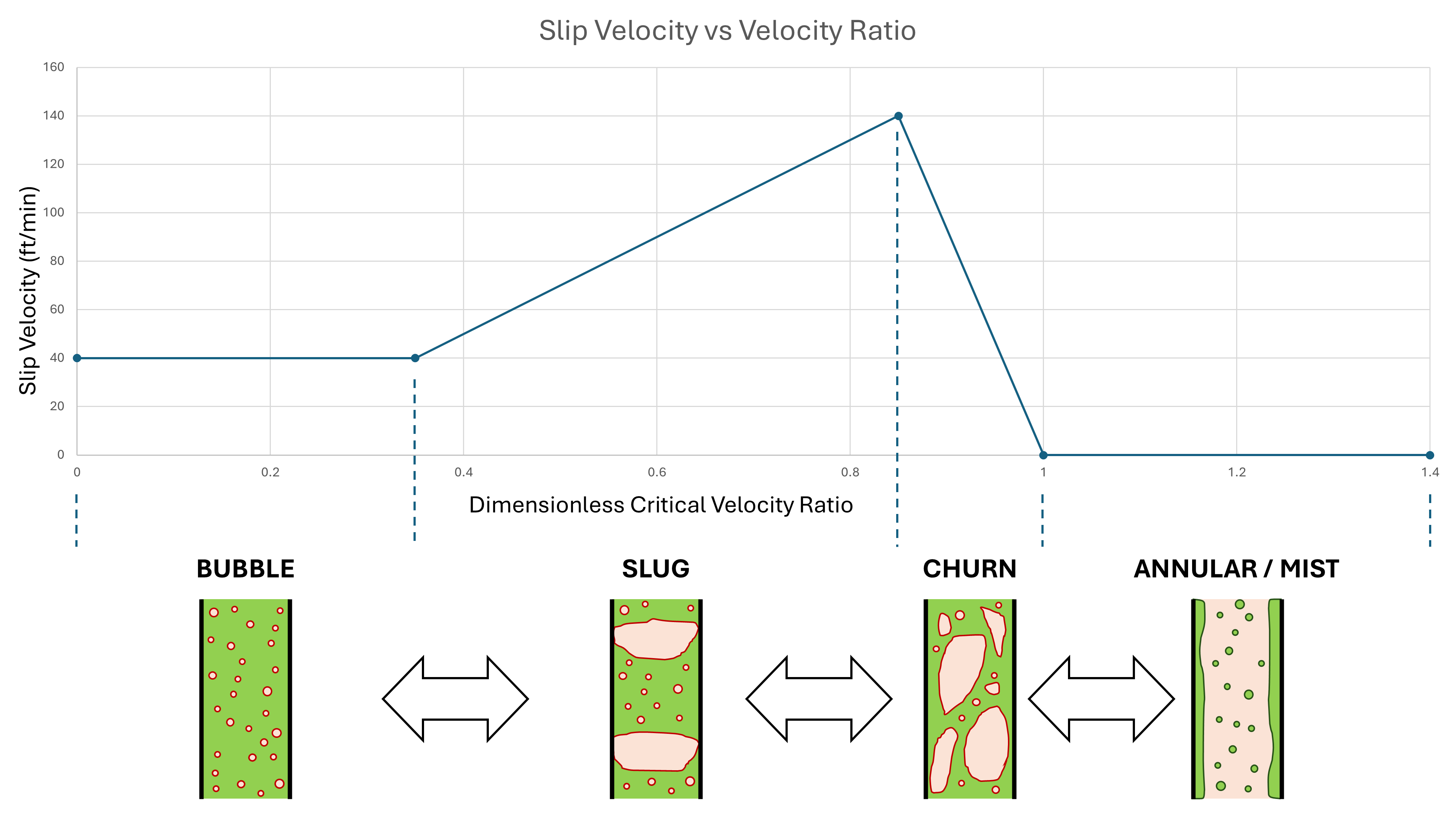
As I have started to learn more about multiphase flow, I have become aware that this hard-coded formulation to obtain \(v_{slip}\) from \(v_{R}\) means the slip is always zero or positive. The concept of negative slip is not handled, although that has been observed in the real world, as highlighted in this LinkedIn post by Dr. Anand Nagoo. This just serves to highlight that the classical approach has shortcomings.
The final step in calculating our hydraulic pressure gradient is to determine the liquid holdup. This is calculated from the superficial velocities of liquid and gas, and the slip velocity itself. It is stated that:
\[v_{slip} \cdot H_{L}^2 + (v_{mix} - v_{slip}) \cdot H_{L} - v_{sL} = 0\]For \(v_{slip} = 0\) this equation reduces to:
\[H_{L} = \frac{v_{sL}}{v_{mix}}\]For other flow regimes, the quadratic equation can be solved to give:
\[H_{L} = \frac{-(v_{mix} - v_{slip}) + \sqrt{(v_{mix} - v_{slip})^2 + 4 \cdot v_{slip} \cdot v_{sL}}}{2 \cdot v_{slip}}\]Finally, we can apply the liquid holdup to our calculation of the mixture density. However, we must also bear in mind that it is necessary to break the wellbore down into smaller segments (typically ~100 ft) as the pressure and temperature will vary as we move closer to the surface. The varying pressure and temperature will alter the fluid densities and thus their volumes, and potentially allow more solution gas or vaporised oil to emerge as we move to a different point in the two-phase region. The classical approach taken is to calculate the conditions at the inlet and outlet boundaries of one segment, and then use the outlet condition as the inlet condition for the next segment. This is known as a marching algorithm, and it is often performed starting at the wellhead and working down; in Pyrus it is assumed that that reservoir fluids are known (defined as modified black oil fluids), and thus the marching is performed from the bottomhole towards the wellhead.
Classical Frictional Gradient
To determine the frictional pressure gradient, we need some additional inputs. These concern the nature of the pipe (diameter and roughness of the internal surface), and some additional fluid properties (viscosities). When combined with the description of the fluid volumetric fractions and velocities determined in the hydrostatic pressure gradient step, we can calculate the frictional pressure loss that occurs as a result of the fluid flowing along the stationary walls of pipe.
There is a widely accepted empirical solution to this, known as the Darcy-Weisbach equation. This formula goes back over a century and has stood the test of time with respect to its accuracy and universal applicability to a wide range of fluids.
We use equation 2.17 in the Standard API RP14E, described as a simplified Darcy-Weisbach equation from the GPSA databook (1981 Revision) for cylindrical pipe:
\[FPG = \frac{0.0000036 \cdot f_{m} \cdot {W}^2}{d_{i}^5 \cdot \rho_{mix}}\]Where:
- \(FPG\) = frictional pressure gradient (psi/ft)
- \(d_{i}\) = pipe inside diameter (inch)
- \(f_{m}\) = Moody friction factor (dimensionless)
- \(\rho_{mix}\) = mixture gas / liquid density at flowing pressure and temperature (lbm/ft3)
- \(W\) = total liquid + vapour rate (lbm/hr)
Of these variables, the pipe inside diameter should be known, the mixture density was previously defined using the liquid holdup calculation from the hydrostatic pressure gradient step, and the mass flow rate should also be known. This leaves the Moody friction factor as the only unknown.
The Moody friction factor depends on the flow regime that is present in the pipe: laminar, turbulent or a transition between the two. Many measurements have been made to accurately determine the friction factor and Moody plotted these in a handy chart. The usefulness of the chart has led to the friction factor becoming known as the Moody friction factor, although technically it should just be the Darcy-Weisbach friction factor. Moody stated that the accuracy of this chart was ±5% for smooth pipes and ±10% for rough pipes.
The laminar portion of the chart (Re <= 2300) is calculated using:
\[f_{m} = \frac{64}{Re}\]\(Re\) is the dimensionless Reynolds number:
\[Re = \frac{\rho \cdot \left < \left < v \right > \right > \cdot D_{h}}{\mu}\]Where:
- \(\rho\) = fluid density
- \(\left < \left < v \right > \right >\) = average in-situ fluid velocity
- \(D_{h}\) = hydraulic radius = \(4A / P\) or \(d_{i}\) for cylindrical pipe
- \(\mu\) = fluid viscosity
It is necessary at this point to digress slightly and note that Reynolds studied at Queens’ College, Cambridge, where I studied Engineering. This little known piece of trivia was drilled into all undergraduate engineers at Queens’. It is somewhat sobering to realise that over a century later we have not managed to significantly advance the state of fluid flow in pipes to an extent that the Reynolds number has faded into the history books. We are truely standing on the shoulders of giants.
But enough already with my hero-worship of Reynolds. Let’s get back to our friction factor… The critical zone portion of the chart between the laminar and transition to turbulent flow (2300 < Re < 4000) is calculated using:
\[f_{f} = \frac{7.05 \times {10^{-8}}}{Re^{-1.5}}\]Note that this formula is for a Fanning friction factor, so to obtain a Moody friction factor it is necessary to multiply by 4×.
As a quick aside, there are actually two commonly used friction factors: the Fanning friction factor (\(f_{f}\)) and the Moody friction factor (\(f_{m}\)). The Moody friction factor and Fanning friction factor are to all extents and purposes identical, other than their relative quantum. The Moody friction factor is exactly 4× as large as the Fanning friction factor. In the oil and gas industry, the Moody friction factor tends to be used by petroleum engineers (hence its appearance in API RP14E), whereas chemical process engineers tend to use equations based around the Fanning friction factor. Quite why this discrepancy arose is a mystery, but it is suffice to note that care should always be taken to ensure the correct friction factor is being used.
For computational purposes the turbulent portion of the Moody chart was captured into an equation by Colebrook and White (1939):
\[\frac{1}{\sqrt{f_{m}}} = -2\log{\frac{\varepsilon}{3.7D_{h}} + \frac{2.51}{Re\sqrt{f_{m}}}}\]Where:
- \(\varepsilon\) = pipe roughness (typically 0.00156 inch for production tubing)
The Colebrook and White equation is implicit in \(f_{m}\) which appears on both sides of the equation. It can be solved iteratively, or solved exactly using the Lambert W formula. In practice, a large number of explicit approximations to the Colebrook-White formula have been proposed. We use the Vatankhah (2014) implementation which was found to have the lowest error across the entire range of the Moody diagram when reviewed and tested by Zeghadnia et al (2018):
\[f_{m} = \left ( \frac{2.51 / Re + 1.1513\delta}{\delta - (\varepsilon / D_{h})/3.71 - 2.3026\delta log(\delta)} \right )^2\] \[\delta = \frac{6.0173}{Re {\left (0.07(\varepsilon / D_{h}) +Re^{-0.885} \right)}^{0.109}} + \frac{\varepsilon / D_{h}}{3.71}\]The combination of these three laminar, transitional and turbulent equations, allows the friction factor to be calculated for any dimensionless Reynolds number and any pipe roughness.
A further complicating factor concerns multiphase flow. The Darcy-Weisbach equation is based on single-phase flow, but with two or more phases, it is not possible to calculate a single Reynolds number. Again, a number of different two-phase Reynolds numbers have been proposed.
We use the formulation proposed by Ortiz-Vidal et al (2014). In this approach, the mixture Reynolds number defined by Shannak is modified by introducing two-phase flow phenomenology through the inclusion of void-fraction parameters. This approach avoids the need for adopting the no-slip homogeneous assumption of the original method. Their results indicate that the inclusion of void-fraction information in the mixture Reynolds number improves the predictions of friction factor when used directly with correlations obtained from single phase flow hydraulics. Note that the paper uses the void fraction α which is equal to \((1 - H_{L})\). Equations have been re-expressed here to use consistent terminology.
\[Re_{mix} = \frac{\rho_{L}{v_{L}}^2{D_{L}}^2 + \rho_{g}{v_{g}}^2{D_{g}}^2}{\mu_{L}v_{L}D_{L} + \mu_{g}v_{g}D_{g}}\]Where:
- \(D_{L}\) = liquid separate cylinder model equivalent diameter
- \(D_{g}\) = gas separate cylinder model equivalent diameter
Using these equations we can create our own visual representation of the Moody chart.
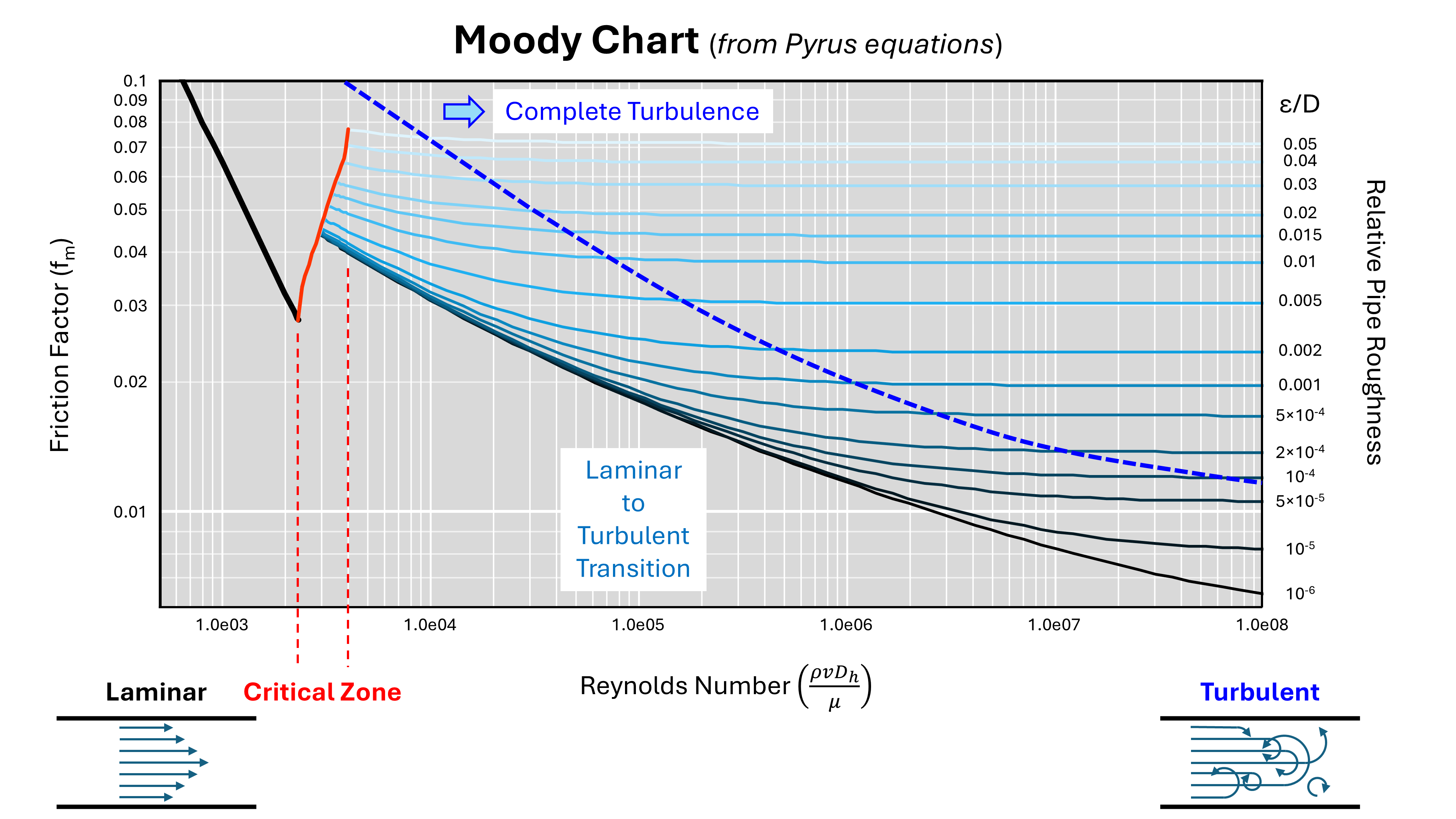
The chart is continuous and matches the published Moody chart with a high degree of accuracy. One difference between the implemented approach and some charts is that in the critical zone, the equation used allows the friction factor to increase gradually from the laminar value to the turbulent value, rather than experiencing a discontinuity at Re = 2,900. This is achieved by using the lower of the critical zone friction factor and the turbulent friction factor between Reynolds number from 2,900 to 4,000.
Classical Kinetic Gradient
In the classical approach implemented, it is usual for the kinetic term to be ignored as it is usually very small. Thus:
\[KPG = 0\]Where:
- \(KPG\) = kinetic pressure gradient (psi/ft)
Fundamental Approach
It should be clear that the classical approach is depends on an accurate determination of the liquid holdup. This affects both the hydrostatic pressure gradient and the frictional pressure gradient (via the two-phase Reynolds number).
However, the calculation of liquid holdup is based on the slip velocity, which is itself derived from knowledge of the flow pattern. In the implementation of the classical approach used by Pyrus, it is the dimensionless critical gas velocity that is used to determine the slip velocity and liquid holdup. This is only a crude estimation of the slip velocity. In other classical approaches, the superficial velocities of liquid and vapour phases or dimensionless groups are used to identify the flow pattern from a map generated from multiple experimental points. Once the flow pattern is identified, this drives the choice of equation to correlate to the liquid holdup.
The logic behind the classical approach is that the liquid holdup is related to the flow pattern. Therefore, identification of the flow pattern is an important first step in the classical approach.
The pipe fractional flow theory proposed by Nagoo (2013) takes a different approach. For a multiphase pipe flow there is conservation of mass, momentum and energy that must be honoured. The principle insight of pipe fractional flow theory is that the in-situ velocities and the volume fractions for each phase are what govern these transport processes in multiphase flow. The flow patterns are simply a manifestation of these parameters. Personally I’ve never liked the approach of first identifying flow patterns. It seems so backwards and overly complicated. With the fundamental approach we can put the flow pattern to the side, and instead focus on how mass, momentum and energy relate to velocity, volume, pressure and temperature. Of course, in Pyrus the equation of state is at the heart of how these parameters relate to each other.
As explained by Nagoo (2013) in his dissertation:
“What is shown in this work is that the real power of the fractional flow graph lies in its ability to generate single-path or multiple-path traverses connecting different flow patterns (thus capturing the connections between different flow phenomena), regardless of whether those paths correlates data on a straight line or not.” (Nagoo, 2013)
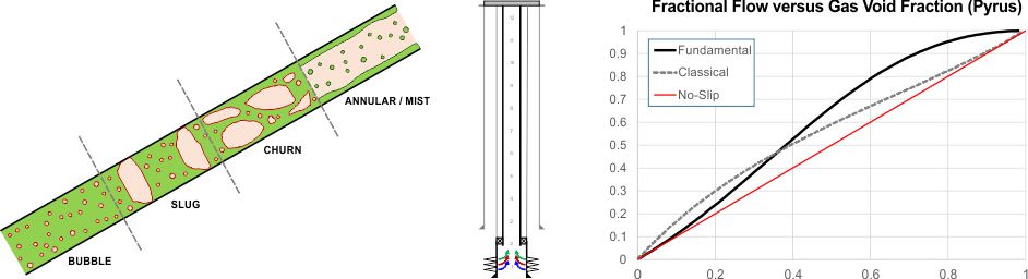
Through analytical methods, it can be shown that there exists a smooth and continuous fractional flow curve that extends across all different flow patterns. In Figure 5 below an analytical fractional flow curve from the fundamental approach is shown against the no-slip assumption (vapour and liquid move at the same velocity), and the implied equivalent flow curve using the classical approach.
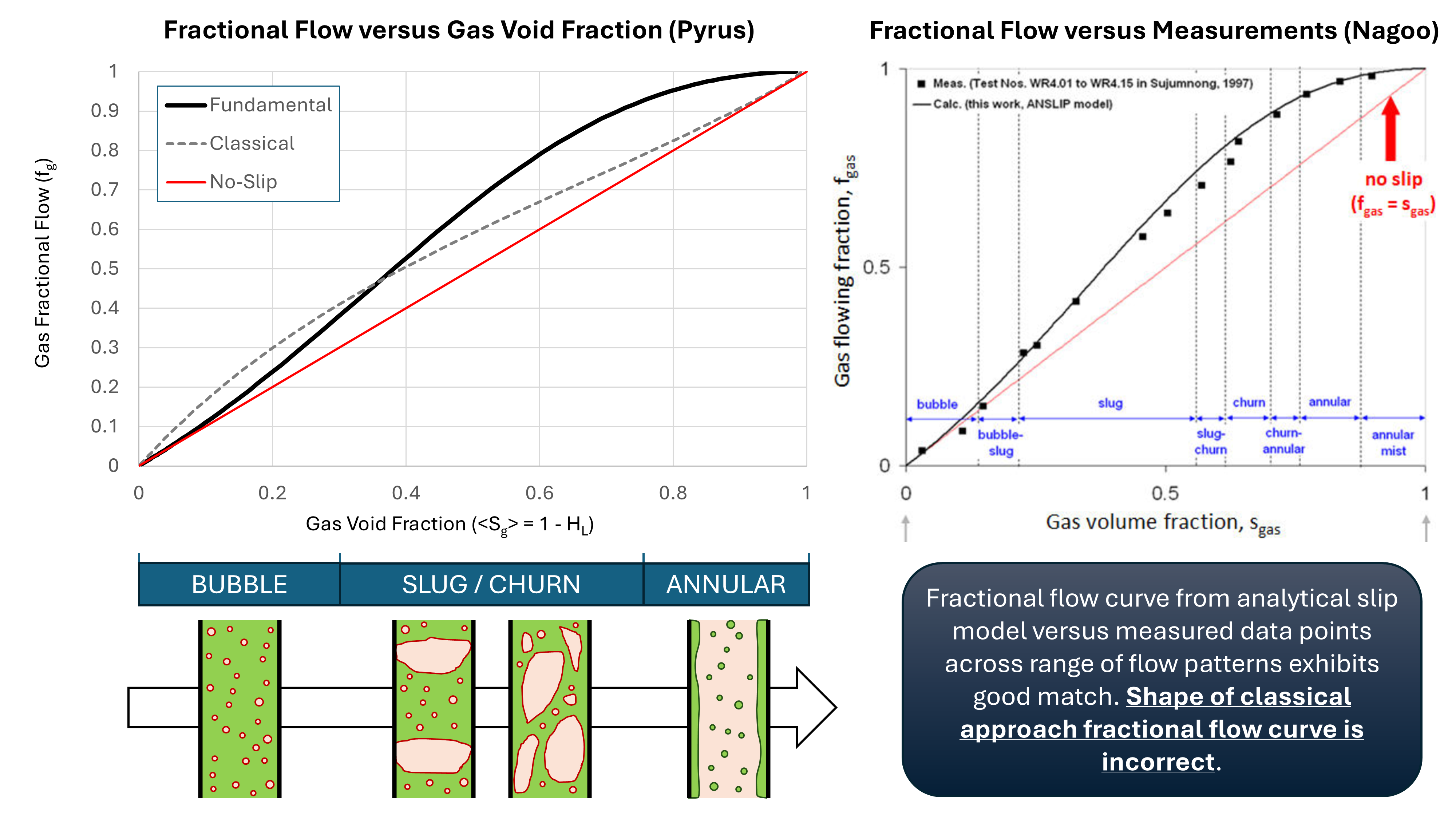
The difference between the fundamental and classical approaches can clearly be seen. Nagoo notes that the fractional flow curves have been tested against 80,000+ datasets and exhibit good predictive qualities. Clearly this is not the case for the implied classical fractional flow curve that emerges as the shape of the curve (left-hand chart in Figure 5) is fundamentally different to that created by the fundamental approach, and which is similar to Nagoo’s comparison of a fraction flow curve against experimental data (right-hand chart in Figure 5).
NOTE: Dr. Nagoo has continued to improve the pipe fractional flow theory, and a much improved version is available in his own software solution. If multiphase fluid flow in pipes is a critical issue for you, then this would be worth investigating further. The version I’ve implemented in Pyrus is an ‘older’ incarnation of the theory (even so I think it is still more logical, versatile and applicable than the classical approach).
Fundamental Hydrostatic Gradient
The fundamental hydrostatic gradient is calculated in the same manner as used in the classical approach. The difference lies in how the liquid holdup is calculated.
The first step involves the definition of a dimensionless relative velocity \(\Omega\). This dimensionless number incorporates all of the average in-situ phase velocities:
Where:
- \(\Omega_{2, 1}\) = dimensionless relative velocity of dispersed phase 2 (vapour) to continuous phase 1 (liquid)
- \(\left < \left < v_{2} \right > \right >\) = averaged in-situ phase 2 (vapour) velocity at any cross-sectional plane, A. This is equivalent to \(v_{g}\).
- \(\left < \left < v_{1} \right > \right >\) = averaged in-situ phase 1 (liquid) velocity at any cross-sectional plane, A. This is equivalent to \(v_{L}\).
- \(\left < u_{mix} \right >\) = averaged mixture volume flux at any cross-sectional plane, A. This is equivalent to \(v_{mix}\) = \(v_{sg} + v_{sL}\).
By expressing velocity for phase-j, \(\left < \left < v_{j} \right > \right >\), as the superficial velocity:
\[\left < u_{j} \right > = \left < \left < v_{j} \right > \right > \left < S_{j} \right > = \frac{q_{j}}{A}\]And substituting the gas phase flowing fraction:
\[f_{2} = \frac{\left < u_{2} \right >}{\left < u_{mix} \right >} = \frac{\left < u_{2} \right >}{\left < u_{1} \right > + \left < u_{2} \right >}\]The dimensionless relative velocity can be re-arranged to yield:
\[f_{2} = \left ( 1 + \left ( 1 - \left < S_{2} \right > \right ) \Omega_{2, 1} \right )\left < S_{2} \right >\]Where:
- \(\left < S_{2} \right >\) = phase 2 (vapour) volume fraction. This is equivalent to the gas void fraction \(H_{g} = 1 - H_{L}\).
Nagoo (2013) shows that many averaged volume fraction correlations can be represented using this fractional flow framework. Furthermore, a wholly analytical closure model that describes the averaged volume fractions is derived. This relationship does not rely on any correlations and is implicit in its flow pattern (e.g., no a priori knowledge of the flow pattern is required). This is referred to as the “ANSLIP” model (analytical slip model). ANSLIP is only recommended for vapour-liquid flows in horizontal, up-inclined and vertical pipe. For vapour-liquid down-inclined flow, or liquid-liquid and fluid-solid flows, other slip models are recommended.
The premise is that the dimensionless relative velocity of the dispersed gas phase (\(\Omega_{2, 1}\)) is equal to the gas phase flowing fraction (\(f_{2}\)).
Thus:
\[f_{2} = \frac{\left < S_{2} \right >}{1 - \left < S_{2} \right > \left ( 1 - \left < S_{2} \right > \right )}\]The ANSLIP model was found to be “very accurate over an enormous range of different concurrent flow applications and flow patterns”.
Furthermore, the ANSLIP model can be re-arranged to directly calculate the gas void fraction or liquid holdup:
\[\left < S_{2} \right > = \frac{f_{2} + 1 - \sqrt{ {\left ( f_{2} + 1 \right )}^2 - 4 \cdot {\left ( f_{2} \right )}^2} }{2 \cdot \left ( f_{2} \right )}\]This is straightforward to solve. Recall that \(\left < S_{2} \right > = 1 - H_{L}\) and \(f_{2} = v_{sg} / (v_{sL} + v_{sg})\). Given the absence of slip velocities, slip ratios, flow patterns etc. the claim that the ANSLIP model “is the simplest and most consistently accurate, analytical annular flow model to date” appears to be something of an understatement.
In practice there is another step that I won’t go into detail on here, which relates to entrainment, whereby liquid droplets from an annular film are entrained into the flow gas phase in the pipe core. Nagoo (2013) also considers the principle of bi-directional two-phase entrainment. In this phenomenon, during the entrainment of phase 1 into phase 2, simultaneously, the corrected phase 2 will itself be entraining back into the continuously diminishing phase 1. The entrainment calculations are handled in Pyrus, but are something of a distraction when considering the overall implications of pipe fractional flow theory, so they will not be discussed further here.
Fundamental Frictional Gradient
The fundamental approach goes back to first principles. No hacks or empirical correlations. Just physics.
Let’s recall the fundamental Darcy-Weisbach equation:
\[FPG = \frac{f_{m} \cdot \rho \cdot {\left < \left < v \right > \right >}^2}{2 \cdot D_{h}}\]This can be re-expressed in terms of a summation of individual phases:
\[FPG = \left ( \frac{1}{2 \cdot D_{h}} \right ) \cdot \left( \frac{f_{m,1} \cdot \rho_{1} \left | \left < u_{1} \right > \right | \cdot \left < u_{1} \right >}{ {1 - \left < S_{2} \right >}^2 } + \frac{f_{m,2} \cdot \rho_{2} \left | \left < u_{2} \right > \right | \cdot \left < u_{2} \right >}{ {\left < S_{2} \right >}^2 } \right )\]In contrast to the classical approach which uses a simplified Darcy-Weisbach equation and relies on calculation of a two-phase Reynolds number for the mixture, in the fundamental approach we calculate the contribution of each phase to the friction. This means that we must instead use the in-situ Reynolds numbers when calculating the Moody friction factor for each of the phases:
\[Re_{j} = \frac{\rho_{j} \left | \left < u_{j} \right > \right | D_{h}}{\mu_{j} \left < S_{j} \right >}\]All terms here are determined either from the previous hydrostatic step, or from an equation of state for each fluid at the current segment pressure and temperature.
Fundamental Kinetic Gradient
In the fundamental method we don’t ignore the kinetic term.
This is given as:
\[KPG = \frac{G_{j} \cdot \Delta \left( \frac{G_{j}}{\rho_{j} \left < S_{j} \right >} \right )}{\Delta L}\]Where:
- \(G_{j}\) = averaged phase-j mass flux = \(\rho_{j} \left < u_{j} \right >\)
All terms have previously been calculated. Since we are using a marching algorithm, we can determine the term \(\Delta \left( \frac{G_{j}}{\rho_{j} \left < S_{j} \right >} \right )\) by considering the values calculated at the prior segment and their difference to the values at the current segment.
Total Pressure Gradient
Determination of the total pressure gradient (\(TPG\)) is no more complicated than addition of the hydrostatic, frictional and kinetic components:
\[TPG = HPG + FPG + KPG\]Wellbore Temperature Modelling
The classical and fundamental approaches described determine the \(\Delta P\) for each pipe segment. This allows a pressure profile to be calculated over the entire wellbore. However, our equation of state requires pressure and temperature to determine properties such as density and viscosity for the liquid and vapour phases. How do we go about calculating the wellbore temperature profile?
There are two very simple assumptions that could be used:
- Constant fluid temperature: The fluid temperature entering the wellbore remains constant from bottom hole to wellhead. This is unrealistic, but for very high flow rate liquid production (where the liquid has a high specific heat capacity), it might be a reasonable approximation.
- Geothermal gradient: The subsurface environment has a geothermal gradient and another approach might be to assume that the wellbore temperature equals the subsurface geothermal gradient. This is also unrealistic, but for very low flow rate gas production, it might be a reasonable approximation since the gas will quickly approach the temperature of the subsurface environment.
What is really needed is an approach that falls somewhere in between these two assumptions.
Pyrus implements the approach described by Sagar, Doty and Schmidt (1991) which is based on a model derived from the steady-state energy equation, taking into consideration all the heat transfer mechanisms that are encountered in a wellbore. These mechanisms include: (1) radial heat conduction through the tubing, annulus, casing and cement into the surrounding earth environment, (2) Joule-Thomson heating or cooling effects caused by pressure changes as the fluid flows up the well, and (3) kinetic energy term.
The ordinary differential equation that describes the change in fluid temperature for a change in length along the wellbore is:
\[\frac{dT_f}{dL} = -A \left [ \left ( T_f - T_e \right ) + \frac{g}{g_c} \cdot \frac{\sin\theta}{J \cdot C_{pm}A} - \frac{F_c}{A} \right ]\]Where:
- \(T_f\) = flowing fluid temperature (°F)
- \(A\) = coefficient (ft-1)
- \(T_e\) = surrounding earth temperature (°F)
- \(g\) = gravitational acceleration (32.2 ft/sec2)
- \(g_c\) = unit conversion factor (32.2 ft-lbm/sec2-lbf)
- \(\theta\) = angle of inclination (degrees)
- \(J\) = mechanical equivalent of heat (778 ft-lbf/Btu)
- \(C_{pm}\) = specific heat of mixture (Btu/lbm-°F)
- \(F_c\) = combination of Joule-Thomson and kinetic energy terms into a single correlation factor
In Sagar, Doty and Schmidt (1991), a correlation is used to estimate the combined Joule-Thomson effect and kinetic energy contribution to the temperature profile. In Pyrus we can dispense with the correlation (which has a limited range of applicability) and determine these values exactly after obtaining the necessary variables from an equation of State. We calculate the correlation factor as:
\[F_C = \mu\frac{dP}{dL} - \frac{v \cdot dv}{J \cdot g_c \cdot C_{pm}}\]Where:
- \(\mu\) = Joule–Thomson coefficient
- \(dP/dL\) = change in pressure over length of well segment (psi/ft). This is our total pressure gradient (\(TPG\)).
- \(v\) = fluid velocity (ft/sec)
The coefficient \(A\) is given as:
\[A = \frac{2\pi}{C_{pm}w_t} \left [ \frac{r_{ti}Uk_e}{k_e + f(t)r_{ti}U} \right ]\]Where:
- \(U\) = overall heat transfer coefficient (Btu/D-ft2-°F)
- \(k_e\) = thermal conductivity of earth (Btu/D-ft-°F). Sagar et al. suggest that, for most geographical areas, this this ~1.4 Btu/D-ft-°F.
- \(f(t)\) = dimensionless transient heat conduction time function for earth
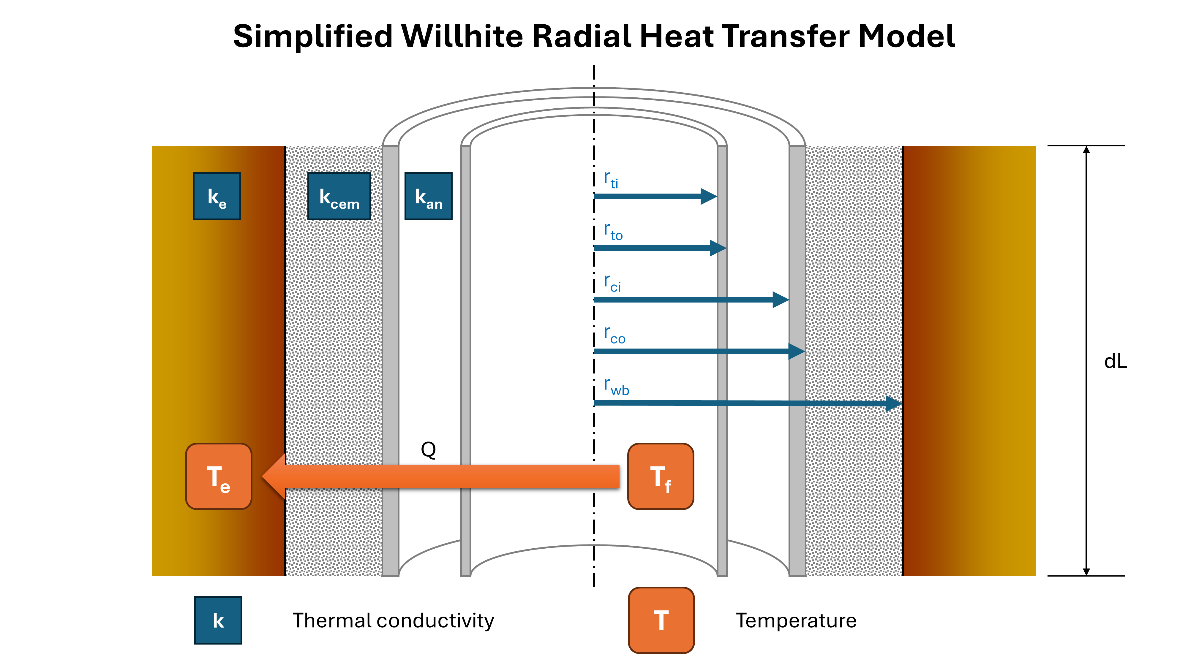
Determination of the overall heat transfer coefficient depends on the configuration of the wellbore tubulars, and it is noted by Sagar et al. that this can be a difficult and critical step in finding an accurate solution. Detailed theoretical equations to calculate the overall heat-transfer in terms of natural convection, conduction and radiation have been proposed by Willhite (1967) and Bird et al. (2002). By neglecting the radiation and convection terms, and assuming that the thermal conductivity of the steel tubing and casing is effectively infinite (negligible thermal resistance in comparison to annulus fluids, cement and earth), the Willhite equation can be expressed as:
\[U = {\left [ r_{ti}\frac{\log_{e}(r_{ci}/r_{to})}{k_{an}} + r_{ti}\frac{\log_{e}(r_{wb}/r_{co})}{k_{cem}} \right ]}^{-1}\]Where:
- radii are inner and outer tubing and casing radii, plus wellbore as per Figure 6 (inch)
- \(k_{an}\) = thermal conductivity of fluid in annulus (Btu/D-ft-°F)
- \(k_{cem}\) = thermal conductivity of cement (Btu/D-ft-°F)
Finally we need to estimate the transient time function. We approximate this as the long-time solution to the radial heat conduction problem for an infinitely long cylinder. The equation is:
\[f(t) = \log_{e} \left [\frac{2 \sqrt{\alpha \cdot t}}{(r_{wb} / 12)} \right ] - 0.29\]Where:
- \(\alpha\) = thermal diffusivity of earth (0.04 ft2/hr)
- \(t\) = time (days). 7 days is a reasonable assumption.
Integration of the ordinary differential equation over a fixed length pipe segment allows the outlet temperature to be determined from the inlet temperature. This is particularly useful for a marching algorithm where the conditions for each successive segment are determined sequentially. To solve the integration, it is assumed that the following values are constant over the segment interval: (1) correlation factor, \(F_c\), (2) relaxation distance, \(A\), (3) geothermal gradient, \(g_G\), (4) specific heat, \(C_{pm}\), (5) inclination angle, \(\theta\). Provided these parameters are approximately constant over the interval in question, there is no other restriction on the length interval that can be used (e.g., this could potentially be the entire well measured depth). In practice, the same segment lengths that are used for the multiphase pressure solution are applied. The outlet fluid temperature \(T_f\) can be determined:
\[T_f = T_e - \frac{g}{g_c} \cdot \frac{\sin\theta}{J \cdot C_{pm}A} + \frac{F_c}{A} + \frac{g_G \cdot \sin\theta}{A} + e^{-A(L - L_{in})} \left ( T_{fin} - T_{ein} + \frac{g}{g_c} \cdot \frac{\sin\theta}{J \cdot C_{pm}A} - \frac{F_c}{A} - \frac{g_G \cdot \sin\theta}{A} \right )\]Where inlet conditions:
- \(L_{in}\) = distance from perforations at pipe segment inlet (ft)
- \(T_{fin}\) = fluid temperature at pipe segment inlet (°F)
- \(T_{ein}\) = earth temperature at pipe segment inlet (°F)
Iterating to Create a Profile
All the necessary steps to create a temperature and pressure profile for a well have been described above. These can be used together to generate a flowing wellbore condition profile, from perforations to the wellhead.
There are two main inputs that are needed:
- Accurate description of the wellbore geometry. This includes the trajectory, tubing and casing sizes and lengths. At a minimum, for every depth point, the casing diameter for the innermost casing string that is cemented and the pipe diameter in which flow is taking place (typically tubing) is required.
- Description of the reservoir fluids produced into the wellbore. We use a modified black-oil model where the reservoir gas can contain vaporised oil that condenses as pressure and temperature drops below dewpoint, and the reservoir oil can contain solution gas which effervesces as pressure and temperature drops below bubblepoint. Hydrocarbons must be described compositionally as a cubic equation of state is used to flash the produced hydrocarbons at the temperature and pressure in each pipe segment. If composition is not available, it can be estimated using the genetic algorithm composition estimation tool in Pyrus. The water properties are also needed.
The algorithm used breaks the wellbore down into approximately 100 ft pipe segments. Figure 7 shows the calculation steps for each segment. The first segment considered is at the perforations depth. The pressure is the FBHP needed to achieve the desired production rate, and the temperature is the reservoir temperature (gas may need to be adjusted for Joule-Thomson effect).
Fluid properties are determined for two combined liquid and vapour phases. The vapour phase comprises the average properties determined for the flashed gas and solution gas, and the liquid phase comprises the average properties determined for the flashed oil and vaporised oil plus water.
Using the classical or fundamental approach, the hydrostatic, frictional and kinetic pressure gradients are determined. These are added up and multiplied by the pipe segment length to obtain the pressure differential (usually a loss in pressure), from which the outlet pressure is calculated.
The temperature differential is calculated next. The pressure differential influences whether there is any Joule-Thomson cooling or heating to account for, and the fluid properties are calculated for the current inlet temperature and pressure to ascertain the Joule-Thomson coefficient and specific heat. These values are used to determine the outlet temperature.
Now the outlet temperature and pressure become the inlet conditions for the next pipe segment. Our modified black oil compositions are flashed again at these new conditions to determine the new set of averaged fluid properties.
Rinse and repeat until the last pipe segment is reached at the wellhead.
Next Steps
The steps described in this blog post have been implemented into Pyrus, and the code is currently being used to test the algorithm performance against published datasets as part of the #100ProductionDatasetsChallenge that is being put together by Dr. Anand Nagoo.
This is an interesting challenge as it is essentially doing a blind test on the predictive capabilities of Pyrus against other established commerical software tools. There is a good chance that the results from Pyrus will be horrifically poor. Yet even if this is the case, it will provide a rare opportunity to discover where the weaknesses are, and to improve the algorithms.
References
- API RP 14, Recommended Practice for Design and Installation of Offshore Production Platform Piping Systems, fifth edition. 1991. Washington, DC: API.
- Bird, R. B., Stewart, W. E., and Lightfoot, E. N. 2002. Transport Phenomena, second edition. New York City: John Wiley and Sons Inc.
- Colebrook, C.F. 1939. Turbulent Flow in Pipes, with Particular Reference to the Transition Region Between the Smooth and Rough Pipe Laws. J Inst Civ Eng 11 (04): 133-156. https://doi.org/10.1680/ijoti.1939.13150.
- Moody, L. F. 1944. Friction Factors for Pipe Flow. In Transactions of the ASME 66 (08): 671–684.
- Nagoo, A. 2013. Pipe Fractional Flow Theory: Principles and Applications. PhD dissertation, The University of Texas at Austin, Texas (December 2013).
- Ortiz-Vidal, L. E., Mureithi, N. and Rodriguez, O. M. H. 2014. Two-Phase Friction Factor in Gas-Liquid Pipe Flow. Revista De Engenharia Térmica 13 (02): 81-88. https://doi.org/10.5380/reterm.v13i2.62101.
- Sagar, R., Doty, D. and Schmidt Z. 1991. Predicting Temperature Profiles in a Flowing Well. SPE Prod Eng 6 (04): 441-448. SPE-19702-PA. https://doi.org/10.2118/19702-PA.
- Turner, R. G., Hubbard, M. G. and Dukler, A. E. 1969. Analysis and Prediction of Minimum Flow Rate for the Continuous Removal of Liquids from Gas Wells. J Pet Technol 21 (11): 1475–1482. https://doi.org/10.2118/2198-PA.
- Vatankhah, A. R. 2014. Comment on “Gene Expression Programming Analysis of Implicit Colebrook-White Equation in Turbulent Flow Friction Factor Calculation”. J Petroleum Sci Eng 124 (December 2014): 402–405. https://doi.org/10.1016/j.petrol.2013.12.001.
- Willhite, G. P. 1967. Over-all Heat Transfer Coefficients in Steam and Hot Water Injection Wells. J Pet Technol 19 (05): 607-615. https://doi.org/10.2118/1449-PA.
- Zeghadnia, L., Robert, J. L. and Achour, B. 2019. Explicit Solutions For Turbulent Flow Friction Factor: A Review, Assessment And Approaches Classification. Ain Shams Engineering Journal 10 (2019): 243-252. https://doi.org/10.1016/j.asej.2018.10.007.