Two popular gas viscosity methods used in the oil and gas industry were both first proposed in the 1960s. These are the Lee, Gonzalez and Eakin (LGE) correlation, and the Lohrenz, Bray and Clark (LBC) correlation. Both have found widespread acceptance and usage.
Recently a new approach for high-level gas viscosity prediction was published. This only requires knowledge of the gas specific gravity, and the inerts content with respect to carbon dioxide, hydrogen sulphide, nitrogen, and hydrogen mole fractions. The method leverages the Peng-Robinson equation of state, but since the objective is to find properties for a single phase (gas), there is no need to iterate to a two-phase solution. This makes application of the cubic solution far easier than other viscosity implementations. Even in comparison to other iterative viscosity solutions such as Dranchuk and Abou-Kaseem (DAK) or Hall and Yarborough (HY) which are iterative algorithms for the Standing and Katz generalised Z-factor chart, the solution provided is explicit and should not have any convergence issues that can sometimes plague DAK and HY.
Burgoyne-Nielsen-Stanko Method
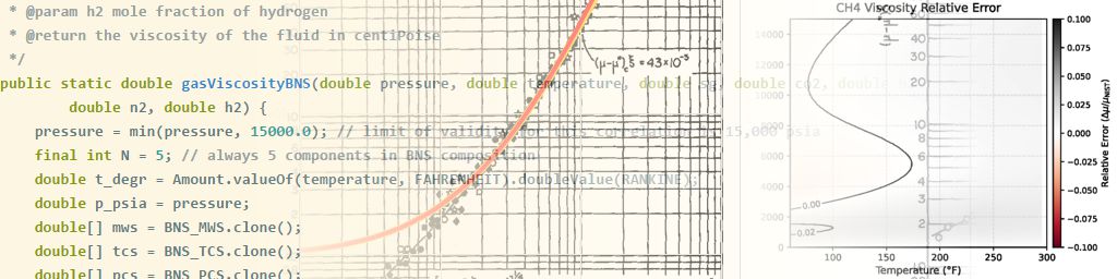
The LBC viscosity method is based on the observation that the residual viscosity multiplied by a viscosity reducing factor is related to the reduced density of a fluid. LBC uses the relationship of Jossi, Stiel and Thodos (JST) (1962) and this is shown in Figure 1 below. By determining the reduced density, it is thus possible to obtain the viscosity of a fluid.
For a gas, the density is related to the volume of the fluid through the real gas law:
\[PV=znRT\]Where (in oilfield units):
- P = pressure (psia)
- V = volume (ft3)
- z = gas-deviation (Z) factor
- n = number of lbm-mol
- R = gas constant = 10.731557089016 (psia·ft3) / (lbm-mol·°R)
- T = temperature (°R)
The Peng-Robinson cubic equation of state defines this as:
\[P=\frac{RT}{V-b}-\frac{a}{V(V+b)+b(V-b)}\]Through use of mixing rules for the various components, the a and b values are combined to obtain mixture equivalents A and B from which the Z-factor can be expressed as:
\[z^3+(B-1)z^2+(A-3B^2-2B)z+(B^3+B^2-AB)=0\]This means that if we solve the Peng-Robinson equation for z, we can obtain the reduced density and apply LBC to in turn obtain the viscosity. Usually solving a cubic equation of state requires determining how many roots exist in the cubic solution, and applying a successive substitution method to determine k-values with Rachford-Rice and fugacities so that the compositions for the liquid and vapour phases can be found. The key insight from Burgoyne et al. is that if we know we have a single phase gas, then we can just select the largest root and no repetitive flash calculations are required. As a consequence the solution for the cubic is massively simplified for implementation in spreadsheets and simple programs. It effectively becomes an explicit function.
Calculation Procedure
The BNS method involves more than just a single equation. Several steps are involved, although none is itself overly complex. Each step is as follows:
-
Define mole fraction composition.
The composition used for the BNS method is a five component mixture. The components, in index order for the arrays, are carbon dioxide (CO2), hydrogen sulphide (H2S), nitrogen (N2), hydrogen (H2) and a pseudo-hydrocarbon. The pseudo-hydrocarbon must have the same specific gravity as the gas mixture.
-
Override pseudo-hydrocarbon Tc, Pc.
Override pseudo-hydrocarbon Tc, Pc using BNS correlations into arrays of tuned critical temperatures and pressures. In developing the BNS method, several existing pseudocritical property calculation methods were tested. It is reported that none of these were able to recreate the Z-factors in the Standing and Katz chart. It was also observed that several pseudocritical property methods actually fail to honour the critical properties of methane when there are no inerts in the mixture and the specific gravity is set to that of methane. To address this, Burgoyne et al. developed new correlations for the critical temperature and pressure.
Burgoyne et al. also created two different correlations for associated gas and for gas-condensate. The implemented approach in the open-source code appears to be assume gas-condensate by default, unless associated gas is specified. If the type of gas is not known, but a mixture composition is available, then it is noted that the regressions were created on the basis that if the C7+/C2 mole fraction ratio is above 0.65, then this was classified as an associated gas. This same logic is applied in Pyrus if using the BNS method with a gas mixture composition.
The pseudocritical properties are given by:
\[T_c=\frac{a\cdot\Delta{MW}}{b+\Delta{MW}}+c \label{eq:bns_eq6}\] \[P_c=\frac{RT_c}{\left(\frac{V_c}{z_c}\right)} \label{eq:bns_eq7}\]With:
\[\frac{V_c}{z_c}=Slope_{V_c}\cdot\Delta{MW}+{\left(\frac{V_c}{z_c}\right)}_{CH_4} \label{eq:bns_eq8}\] \[\Delta{MW}=MW_{Hydrocarbon}-MW_{CH_4} \label{eq:bns_eq9}\]Constants in equation \ref{eq:bns_eq6} are given by:
Parameter Gas-Condensate Associated Gas a 1098.1095 2695.1477 b 101.5292 274.3417 c \({T_{crit}}_{CH_4}\) \({T_{crit}}_{CH_4}\) Slopevc 0.170931 0.177498 Methane critical components are given as:
\({T_{crit}}_{CH_4}\) (°R) \({P_{crit}}_{CH_4}\) (psia) \({\left(\frac{V_c}{z_c}\right)}_{CH_4}\) (ft3/lbm-mol) \({MW}_{CH_4}\) (lbm/lbm-mol) 343.008 667.029 5.518526 16.0425 -
Calculate temperature-dependent BIPs.
Calculate temperature-dependent pairs of binary interaction parameters (BIPs) for the kij matrix used in the mixing rule to obtain A in the Peng-Robinson equation. The BIPs are evaluated at the temperature of interest using Tc of pseudo-hydrocarbon. This is done to improve the model predictability of mixtures in single phase conditions close to the saturation region. The BIPs were determined by matching experimental data from published literature sources.
Each component-pair BIP kij is given by:
\[k_{ij}=a+\frac{b}{T_{rSolvent}}\]Where:
Component-Pair a b \(T_{rSolvent}\) Hydrocarbon : CO2 -0.14556 0.276572 Equation \ref{eq:bns_eq6}, \ref{eq:bns_eq9} Hydrocarbon : H2S 0.16852 -0.12238 Equation \ref{eq:bns_eq6}, \ref{eq:bns_eq9} Hydrocarbon : N2 -0.108 0.060551 Equation \ref{eq:bns_eq6}, \ref{eq:bns_eq9} Hydrocarbon : H2 -0.06201 0.042787 Equation \ref{eq:bns_eq6}, \ref{eq:bns_eq9} CO2 : H2S 0.248638 -0.13819 547.416 CO2 : N2 -0.25 0.11602 547.416 CO2 : H2 -0.24715 0.16377 547.416 H2S : N2 -0.20441 0.234417 672.12 H2S : H2 0 0 672.12 N2 : H2 -0.16625 0.078813 227.16 -
Use the PR EOS to solve for Z-factor.
Use the PR EOS to solve for Z-factor analytically at the given P, T. For most spreadsheet style applications, the largest root can be taken as the gas phase Z-factor. In this implementation we apply the same trick as employed by Burgoyne to determine if there are actually three roots. If this is the case then we determine the lowest fugacity coefficient to select the correct root.
For the inert components, the acentric and volume translation factors were tuned to match pure component molar densities against experimental reference data. In addition, ΩA and ΩB were tuned for CO2 and H2S.
Critical and other parameters applied for the PR EOS are:
Parameter CO2 H2S N2 H2 Hydrocarbon-Pseudo MW (lbm/lbm-mol) 44.01 34.082 28.014 2.016 \({T_{crit}}\) (°R) 547.416 672.12 227.16 47.43 Eq \ref{eq:bns_eq6}, \ref{eq:bns_eq9} \({P_{crit}}\) (psia) 1069.51 1299.97 492.84 187.53 Eq \ref{eq:bns_eq7}, \ref{eq:bns_eq8}, \ref{eq:bns_eq9} ACF 0.12253 0.04909 0.03700 -0.21700 -0.03899 VTRAN -0.27607 -0.22901 -0.21066 -0.36270 -0.19076 ΩA 0.427671 0.436725 0.457236 0.457236 0.457236 ΩB 0.0696397 0.0724345 0.0777961 0.0777961 0.0777961 Details for solution of the PR cubic are not given here. The reader is encouraged to study the example code snippets below to understand how this is done.
-
Compute Viscosity using Modified LBC.
Compute the gas viscosity using the LBC method with the adjusted critical volumes and coefficients. The critical volumes (Vcvis), slope and intercept of a new correlation for the hydrocarbon pseudocomponent (Vcvis vs MWHydrocarbon) and the 4th and 5th coefficients of the JST equation were tuned using experimental data for pure fluids and the LGE correlation for hydrocarbon mixtures. The JST equation \ref{eq:residmu_jst} is given as:
\[\left[\left({\mu-\mu^{*}}\right)\xi+10^{-4}\right]^{1/4}=a_1+a_2\rho_r+a_3\rho_r^2+a_4\rho_r^3+a_5\rho_r^4 \label{eq:residmu_jst}\]With:
\[\xi=\frac{[\sum_{i=1}^{n}(z_iT_{ci})]^{1/6}}{[\sum_{i=1}^{n}(z_iM_{i})]^{1/2}[\sum_{i=1}^{n}(z_iP_{ci})]^{2/3}}\]Where:
- μ* = low-pressure mixture gas viscosity (cP)
- (μ − μ*) = residual viscosity (cP)
- ξ = mixture viscosity-reducing parameter ≈ 1 / μc (cP-1)
The tuned coefficients for the BNS implementation of LBC are:
Parameter Normal Fluids a1 0.10230 a2 0.023364 a3 0.058533 a4 -0.0392852 a5 0.00926279 Critical density and reduced density for the mixture are given by:
\[\rho_c=\frac{1}{V_{crit_{vis, mix}}}\] \[\rho_r=\frac{P}{zRT\rho_c}\]Where:
- P = pressure (psia)
- z = gas-deviation (Z) factor
- R = gas constant = 10.731557089016 (psia·ft3) / (lbm-mol·°R)
- T = temperature (°R)
With:
\[V_{crit_{vis, mix}}=\sum_{i=1}^{5}{z_iV_{crit_{vis, i}}}\] \[V_{crit_{vis, hc-pseudo}}=0.057671\cdot\Delta{MW}+1.44383 \label{eq:bns_eq10}\]Parameter CO2 H2S N2 H2 Hydrocarbon-Pseudo \(V_{crit_{vis, i}}\) (ft3/lbm-mol) 1.46352 1.46808 1.35526 0.68473 Eq \ref{eq:bns_eq10}
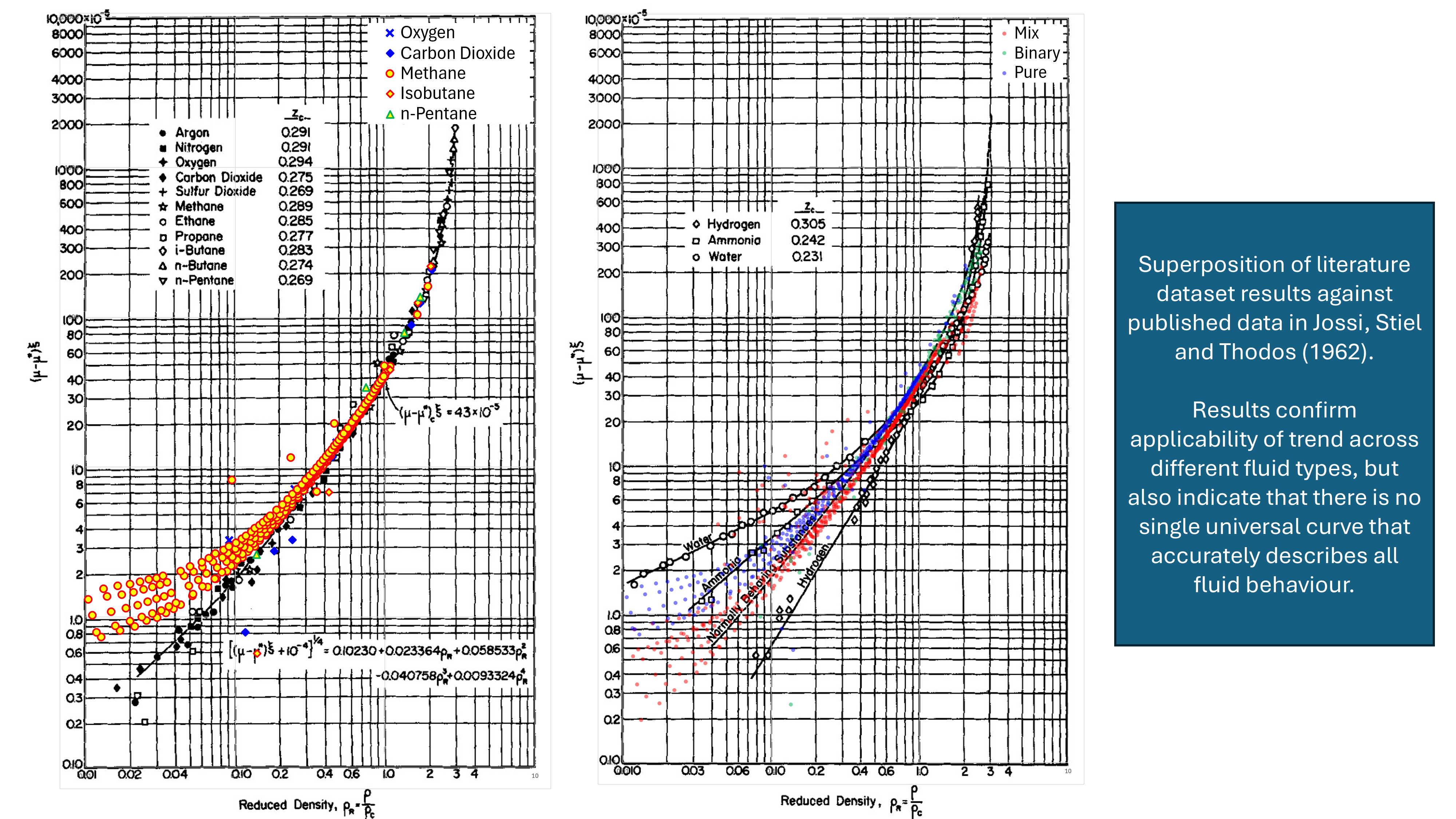
The re-regressed JST relationship versus the original is shown in Figure 2. This shows that the difference is minor and thus deviation from established LBC viscosity correlation is not significant.
Implementation in Java
Mark Burgoyne has provided examples for implementation of BNS code in Visual Basic for Applications (for running in Excel), Python, Fortran and Rust. Shown below are ports of this code (loosely based on the Python implementation for PyResToolbox rather than the code examples) into the Java programming language and with reference to the SPE-229932 paper. Note that this code uses the JScience Amount class, JSR-385 units and custom oilfield units. Further information on the use of generics for strong unit typing in Java is described in this blog post.
In the future I may create a more ‘vanilla’ Java version that omits the unit generics, the FastMap collection (instead of HashMap) and replacing the referencing of pure component properties from the Pyrus library with numerical values. I can then submit a pull request to Mark Burgoyne for the code example to be included with the other languages.
Working backwards, the viscosity is determined as follows:
/**
 * Gas viscosity using tuned Lohrenz–Bray–Clark (BNS implementation). Adjusted critical volumes and coefficients are
 * taken from table 11, equation 10 and table 15 in SPE-229932.
 *
 * @param pressure the gas pressure in psia
 * @param temperature the gas temperature in degrees Fahrenheit
 * @param sg gas specific gravity (air = 1)
 * @param co2 mole fraction of carbon dioxide
 * @param h2s mole fraction of hydrogen sulphide
 * @param n2 mole fraction of nitrogen
 * @param h2 mole fraction of hydrogen
 * @return the viscosity of the fluid in centiPoise
 */
public static double gasViscosityBNS(double pressure, double temperature, double sg, double co2, double h2s,
        double n2, double h2) {
    pressure = min(pressure, 15000.0); // limit of validity for this correlation is 15,000 psia
    final int N = 5; // always 5 components in BNS composition
    double t_degr = Amount.valueOf(temperature, FAHRENHEIT).doubleValue(RANKINE);
    double p_psia = pressure;
    double[] mws = BNS_MWS.clone();
    double[] tcs = BNS_TCS.clone();
    double[] pcs = BNS_PCS.clone();
    double[] vcvis = BNS_VCVIS.clone();
    FluidComponent[] fcs = {PureComponent.CO2, PureComponent.H2S, PureComponent.N2, PureComponent.H2,
        PureComponent.CH4}; // technically last component is a pseudo-hydrocarbon component
    double[] z = {co2, h2s, n2, h2, 1.0 - (co2 + h2s + n2 + h2)}; // build composition vector
    double sg_hc = hydrocarbonSpecificGravity(sg, co2, h2s, n2, h2);
    double hc_gas_mw = sg_hc * PureComponent.AIR.mass();

    // Override pseudo-hydrocarbon MW
    int gas_idx = N - 1; // index 4
    mws[gas_idx] = hc_gas_mw;

    // BNS Tc,Pc for a pure pseudo-hydrocarbon gas (no non-hc components)
    double tpc_hc = criticalTemperatureBNS(sg_hc, 0.0, 0.0, 0.0, 0.0, false); // degR
    double ppc_hc = criticalPressureBNS(sg_hc, 0.0, 0.0, 0.0, 0.0, false); // psia
    tcs[gas_idx] = tpc_hc;
    pcs[gas_idx] = ppc_hc;
    vcvis[gas_idx] = 0.0576710 * (hc_gas_mw - PureComponent.CH4.mass()) + 1.44383; // eq 10 in SPE-229932

    // Dilute gas viscosity from Stiel-Thodos
    FastMap<FluidComponent, Amount<DynamicViscosity>> xi_mui = new FastMap<>(N);
    FastMap<FluidComponent, Double> comp_bns = new FastMap<>(N);
    for (int i = 0; i < N; i++) {
        double tri = t_degr / tcs[i];
        double tc_k = Amount.valueOf(tcs[i], RANKINE).doubleValue(KELVIN);
        double pc_atm = Amount.valueOf(pcs[i], POUND_PER_SQUARE_INCH).doubleValue(ATMOSPHERE);
        double xi = PVT.viscosityReducingParameter(tc_k, pc_atm, mws[i]);
        double mui_cp = PVT.gasViscosityLowPressureStielThodos(tri, xi);
        xi_mui.put(fcs[i], Amount.valueOf(mui_cp, CENTIPOISE));
        comp_bns.put(fcs[i], z[i]);
    }

    // Apply Herning and Zipperer (1936) mixing rule to get mixture dilute gas viscosity.
    Amount<DynamicViscosity> mu_star = mixingRuleHerningZipperer(xi_mui, comp_bns);

    // Determine mixture values that will be used for LBC
    double vcvis_mix = 0.0;
    double tc_k_mix = 0.0;
    double mw_mix = 0.0;
    double pc_atm_mix = 0.0;
    for (int i = 0; i < N; i++) {
        double tc_k_i = Amount.valueOf(tcs[i], RANKINE).doubleValue(KELVIN);
        double pc_atm_i = Amount.valueOf(pcs[i], POUND_PER_SQUARE_INCH).doubleValue(ATMOSPHERE);
        vcvis_mix += vcvis[i] * z[i];
        tc_k_mix += z[i] * tc_k_i;
        mw_mix += z[i] * mws[i];
        pc_atm_mix += z[i] * pc_atm_i;
    }

    // Apply modified LBC form to determine viscosity.
    double rhoc = 1.0 / vcvis_mix;
    double zfac_bns = zFactorBNS(pressure, temperature, sg, co2, h2s, n2, h2);
    double rho_r = p_psia / (zfac_bns * Mixture.GAS_CONSTANT * t_degr * rhoc);
    double xi = PVT.viscosityReducingParameter(tc_k_mix, pc_atm_mix, mw_mix);
    double mu_bns = PVT.viscosityBNSModifiedLBC(rho_r, xi, mu_star.doubleValue(CENTIPOISE));
    return mu_bns;
}

/**
 * Based on method of Jossi, this correlates the residual viscosity to the reduced density but with the last two
 * terms modified by Burgoyne, Nielsen and Stanko (2025). This is specifically used with the BNS viscosity method.
 *
 * @param rho_r reduced density
 * @param xi viscosity reducing parameter (1/cP)
 * @param mu_star dilute gas viscosity at target temperature (cP)
 * @return viscosity at target pressure and temperature in centiPoise
 */
protected static final double viscosityBNSModifiedLBC(double rho_r, double xi, double mu_star) {
    final double[] A_LBC = {0.1023, 0.023364, 0.058533, -0.0392852, 0.00926279};
    double mu = A_LBC[0] + rho_r * (A_LBC[1] + rho_r * (A_LBC[2] + rho_r * (A_LBC[3] + rho_r * A_LBC[4])));
    mu = pow(mu, 4.0);
    mu -= 1.0e-04;
    mu /= xi;
    mu += mu_star;
    return mu;
}
It can be seen near the end that the modified LBC viscosity method relies on the reduced density. In turn this is obtained from the Z-factor which is calculated as follows:
/**
 * Uses BNS tuned Peng Robinson EOS to solve for Z factor. Ported from z_bur at
 * https://github.com/mwburgoyne/pyResToolbox/blob/main/pyrestoolbox/gas/gas.py.
 *
 * @param pressure the gas pressure in psia
 * @param temperature the gas temperature in degrees Fahrenheit
 * @param sg gas specific gravity (air = 1)
 * @param co2 mole fraction of carbon dioxide
 * @param h2s mole fraction of hydrogen sulphide
 * @param n2 mole fraction of nitrogen
 * @param h2 mole fraction of hydrogen
 * @return the Z factor
 */
public static double zFactorBNS(double pressure, double temperature, double sg, double co2, double h2s, double n2,
        double h2) {
    final int N = 5; // always 5 components in BNS composition
    double t_degr = Amount.valueOf(temperature, FAHRENHEIT).doubleValue(RANKINE);
    double p_psia = pressure;
    double[] tcs = BNS_TCS.clone();
    double[] pcs = BNS_PCS.clone();
    double[] acf = BNS_ACF.clone();

    /*
     * Workflow from SPE-229932 for z-factor property calculation is:
     *
     *  1. Define mole fraction composition.
     *  2. Override pseudo-hydrocarbon Tc, Pc using BNS correlations into arrays of tuned critical temperatures and
     *     pressures.
     *  3. Calculate temperature-dependent pairs of BIPs (kij matrix) at temperature of interest using Tc of
     *     pseudo-hydrocarbon.
     *  4. Use the PR EOS to solve for Z-factor analytically at the given P, T. For most spreadsheet style
     *     applications, the largest root can be taken as the gas phase Z-factor. In this implementation we apply
     *     the same trick as employed by Burgoyne to determine if there are actually three roots. If this is the
     *     case then we determine the lowest fugacity coefficient to select the correct root.
     */
    // 1. Define mole fraction composition.
    double[] z = {co2, h2s, n2, h2, 1.0 - (co2 + h2s + n2 + h2)}; // build composition vector

    // 2. Override pseudo-hydrocarbon Tc, Pc using BNS correlations into arrays of tuned critical temperatures and
    //    pressures
    double tpc_hc = criticalTemperatureBNS(sg, co2, h2s, n2, h2, false); // degR
    double ppc_hc = criticalPressureBNS(sg, co2, h2s, n2, h2, false); // psia
    int gas_idx = N - 1; // index 4
    tcs[gas_idx] = tpc_hc;
    pcs[gas_idx] = ppc_hc;

    // 3. Calculate temperature-dependent pairs of BIPs (kij matrix) at temperature of interest using Tc of
    //    pseudo-hydrocarbon.
    double[][] kij = calcBipsBNS(t_degr, tpc_hc);

    // 4. Use the PR EOS to solve for Z-factor analytically at the given P, T. For most spreadsheet style
    //    applications, the largest root can be taken as the gas phase Z-factor.
    // Compute component PR parameters ai, bi.
    double[] ai = new double[N];
    double[] bi = new double[N];
    for (int i = 0; i < N; i++) {
        double tci_degr = tcs[i];
        double tri = t_degr / tci_degr; // component reduced temperature
        double sqrt_tr = Math.sqrt(tri);
        double pci = pcs[i];
        double pri = p_psia / pci; // component reduced pressure
        double omega = acf[i];

        // Standard PR alpha and m(omega).
        double m = 0.37464 + 1.54226 * omega - 0.26992 * omega * omega;
        double alpha = Math.pow(1.0 + m * (1.0 - sqrt_tr), 2.0);
        ai[i] = BNS_OMEGAA[i] * alpha * pri / (tri * tri);
        bi[i] = BNS_OMEGAB[i] * pri / tri;
    }

    // Mixture a_mix (cubic A) and b_mix (cubic B) with BIPs.
    // Mixing rule A: A = dblsum_ij z_i * z_j * sqrt(Ai_i * Ai_j) * (1 - kij)
    // Mixing rule B: B = sum_i z_i * Bi_i
    double a_mix = 0.0;
    double b_mix = 0.0;
    for (int i = 0; i < N; i++) {
        b_mix += z[i] * bi[i];
        for (int j = 0; j < N; j++) {
            double aij = Math.sqrt(ai[i] * ai[j]) * (1.0 - kij[i][j]);
            a_mix += z[i] * z[j] * aij;
        }
    }
    final double A = a_mix;
    final double B = b_mix;

    // Cubic EOS coefficients for PR: Z^3 + c2 Z^2 + c1 Z + c0 = 0
    double c2 = -(1.0 - B);
    double c1 = A - 3.0 * B * B - 2.0 * B;
    double c0 = B * (B * B + B - A);

    // Solve cubic with Halley’s method (single vapour root).
    double z_root = AdvMath.halleyCubic(c2, c1, c0);

    // This is a fugacity-based root selection for sub-critical conditions. When 3 real roots exist, the
    // thermodynamically stable phase is the one with the lowest fugacity coefficient (Gibbs criterion). First we
    // find the discriminant of depressed cubic in order to check for 3 real roots.
    double p_d = (3.0 * c1 - c2 * c2) / 3.0;
    double q_d = (2.0 * c2 * c2 * c2 - 9.0 * c2 * c1 + 27.0 * c0) / 27.0;
    double disc = q_d * q_d / 4.0 + p_d * p_d * p_d / 27.0;

    // If there are three real roots then we are subcritical and must do fugacity-based root selection. Discriminant
    // less than zero implies three real roots.
    if (disc < -1.0e-15) {
        double z_max = z_root;

        // Deflate cubic by z_max to get quadratic for remaining roots.
        double b_q = c2 + z_max;
        double c_q = c1 + z_max * b_q;
        double det = max(b_q * b_q - 4.0 * c_q, 0.0);
        double sqrt_det = Math.sqrt(det);
        double z_min = (-b_q - sqrt_det) / 2.0; // smallest root

        // PR ln(phi) for root selection.
        double sqrt2 = Math.sqrt(2.0);
        double s2p1 = 1.0 + sqrt2;
        double s2m1 = sqrt2 - 1.0;

        // Only compare where z_min is physically valid (Z > B)
        if (z_min > B) {
            double lnphi_max = ((z_max - 1.0)
                    - Math.log(z_max - B)
                    - A / (2.0 * sqrt2 * B)
                    * Math.log((z_max + s2p1 * B) / (z_max - s2m1 * B)));

            double lnphi_min = ((z_min - 1.0)
                    - Math.log(z_min - B)
                    - A / (2.0 * sqrt2 * B)
                    * Math.log((z_min + s2p1 * B) / (z_min - s2m1 * B)));
            if (lnphi_min < lnphi_max) {
                z_root = z_min;
            }
        }
    }

    // Apply volume shift for BNS-style shifted Z
    double vshift_mix = 0.0;
    for (int i = 0; i < N; i++) {
        vshift_mix += z[i] * BNS_VSHIFT[i] * bi[i];
    }
    return z_root - vshift_mix;
}
Several existing functions in Pyrus were used in lieu of re-creating code. In particular the viscosity reducing parameter (ξ) and the Stiel-Thodos low pressure gas viscosity, both of which are needed for the LBC method. The Herning-Zipperer mixing rule was also previously implemented and thus this version was utilised.
/**
 * Component viscosity-reducing parameter ≈ 1 / μci (cP-1).
 *
 * @param tc critical temperature, K
 * @param pc critical pressure, atm
 * @param mw molecular weight, g/mol
 * @return viscosity-reducing parameter ≈ 1 / μci (1/cP)
 */
public static final double viscosityReducingParameter(double tc, double pc, double mw) {
    double xi = pow(tc, 1.0 / 6.0) / (sqrt(mw) * pow(pc, 2.0 / 3.0));
    return xi;
}

/**
 * Calculates the dilute gas viscosity (typically at low pressure 1 to 5 atm) for a component.
 *
 * @param tr reduced temperature
 * @param xi viscosity reducing parameter (1/cP)
 * @return dilute gas viscosity (cP)
 */
public static final double gasViscosityLowPressureStielThodos(double tr, double xi) {
    double mu_star;
    if (tr < 1.5) {
        mu_star = (34.0e-05 * pow(tr, 0.94)) / xi;
    } else {
        mu_star = (17.78e-05 * pow(max(4.58 * tr - 1.67, 1.0e-30), 5.0 / 8.0)) / xi;
    }
    return mu_star;
}

/**
 * In a simplification of the kinetic theory approach, ignoring second order effects, Herning and Zipperer (1936)
 * proposed a viscosity mixing rule based on molecular weights.
 *
 * @param xi_mui map of fluid components to pure component viscosity (allows different pure component viscosities)
 * @param comp map of fluid components to pure component mixture fraction
 * @return viscosity of the mixture
 */
public static Amount<DynamicViscosity> mixingRuleHerningZipperer(
        FastMap<FluidComponent, Amount<DynamicViscosity>> xi_mui, FastMap<FluidComponent, Double> comp) {
    double mui_zi_sqrtmi = 0.0;
    for (FluidComponent fc_i : comp.keySet()) {
        final Double zi = comp.get(fc_i);
        final double m_i = fc_i.mass();
        double zj_phi_ij = 0.0;
        for (FluidComponent fc_j : comp.keySet()) {
            final Double zj = comp.get(fc_j);
            final double m_j = fc_j.mass();
            zj_phi_ij += zj * sqrt(m_j / m_i);
        }
        mui_zi_sqrtmi += (xi_mui.get(fc_i).doubleValue(CENTIPOISE) * zi) / zj_phi_ij;
    }
    return Amount.valueOf(mui_zi_sqrtmi, CENTIPOISE);
}
Helper functions for the viscosity calculation include obtaining the hydrocarbon specific gravity, the critical temperature, and the critical pressure:
protected static double hydrocarbonSpecificGravity(double sg, double co2, double h2s, double n2, double h2) {
    double sg_hc = 0.75; // default value if 100% inerts to avoid numerical problems
    if (co2 + h2s + n2 + h2 < 1.0) {
        final double MW_CO2 = PureComponent.CO2.mass();
        final double MW_H2S = PureComponent.H2S.mass();
        final double MW_N2 = PureComponent.N2.mass();
        final double MW_H2 = PureComponent.H2.mass();
        sg_hc = (sg - (co2 * MW_CO2 + h2s * MW_H2S + n2 * MW_N2 + h2 * MW_H2) / PureComponent.AIR.mass())
                / (1.0 - co2 - h2s - n2 - h2);
        sg_hc = max(PureComponent.CH4.specificGravity(), sg_hc);
    }
    return sg_hc;
}

/**
 * Calculates pseudo-critical temperature for the pseudo-hydrocarbon component. Uses custom linear fits for gas
 * condensates and associated gas (Burgoyne, 2025). These relations are derived from property fitting and may differ
 * from literature.
 *
 * @param sg gas specific gravity (air = 1.0)
 * @param co2 mole fraction of carbon dioxide
 * @param h2s mole fraction of hydrogen sulphide
 * @param n2 mole fraction of nitrogen
 * @param h2 mole fraction of hydrogen
 * @param is_ag flag for if this associated gas (true) or gas-condensate (false)
 * @return the critical temperature for the pseudo-hydrocarbon component in degrees Rankine (degR)
 */
public static double criticalTemperatureBNS(double sg, double co2, double h2s, double n2, double h2,
        boolean is_ag) {
    int idx = is_ag ? 0 : 1;
    double sg_hc = hydrocarbonSpecificGravity(sg, co2, h2s, n2, h2);
    final double[] A = {2695.14765, 1098.10948};
    final double[] B = {274.341701, 101.529237};
    final double[] C = {PureComponent.CH4.t_crit(), PureComponent.CH4.t_crit()};
    double x = max(0.0, PureComponent.AIR.mass() * sg_hc - PureComponent.CH4.mass());
    double tpc_hc = A[idx] * x / (B[idx] + x) + C[idx];
    return tpc_hc;
}

/**
 * Calculates pseudo-critical pressure for the pseudo-hydrocarbon component. Uses custom linear fits for gas
 * condensates and associated gas (Burgoyne, 2025). These relations are derived from property fitting and may differ
 * from literature.
 *
 * @param sg gas specific gravity (air = 1.0)
 * @param co2 mole fraction of carbon dioxide
 * @param h2s mole fraction of hydrogen sulphide
 * @param n2 mole fraction of nitrogen
 * @param h2 mole fraction of hydrogen
 * @param is_ag flag for if this associated gas (true) or gas-condensate (false)
 * @return the critical pressure for the pseudo-hydrocarbon component in psia
 */
public static double criticalPressureBNS(double sg, double co2, double h2s, double n2, double h2, boolean is_ag) {
    int idx = is_ag ? 0 : 1;
    double sg_hc = hydrocarbonSpecificGravity(sg, co2, h2s, n2, h2);
    final double[] VC_SLOPE = {0.177497835, 0.170931432};
    double x = max(0.0, PureComponent.AIR.mass() * sg_hc - PureComponent.CH4.mass());
    double tpc_hc = criticalTemperatureBNS(sg, co2, h2s, n2, h2, is_ag);
    double vc_on_zc = VC_SLOPE[idx] * x + 5.518525872412144;
    double ppc_hc = Mixture.GAS_CONSTANT * tpc_hc / vc_on_zc;
    return ppc_hc;
}
Helper functions for the Z-factor calculation include assembling the binary interaction parameter matrix and solving the cubic equation:
/**
 * Compute 5x5 BIP matrix using precomputed constants. From equation 4 in paper SPE-229932.
 *
 * @param deg_r temperature in Rankine
 * @param tpc_hc pseudo-critical temperature of the gas (same units as BNS_TCS)
 * @return 5x5 kij matrix
 */
private static double[][] calcBipsBNS(double deg_r, double tpc_hc) {
    final int N = 5;
    double[][] slope_tc = new double[N][N];
    for (int i = 0; i < N; i++) {
        System.arraycopy(BIP_SLOPE_TC[i], 0, slope_tc[i], 0, N);
    }
    for (int j = 0; j < 4; j++) {
        slope_tc[4][j] = BIP_GAS_SLOPES[j] * tpc_hc;
    }
    for (int i = 0; i < 4; i++) {
        slope_tc[i][4] = slope_tc[4][i];
    }
    double[][] kij = new double[N][N];
    for (int i = 0; i < N; i++) {
        for (int j = 0; j < N; j++) {
            kij[i][j] = BIP_CONST[i][j] + slope_tc[i][j] / deg_r;
        }
    }
    return kij;
}

/**
 * Halley solver for cubic: x^3 + c2 * x^2 + c1 * x + c0 = 0. Returns the largest real root. Falls back to
 * cubicSolver() if Halley does not converge.
 */
public static double halleyCubic(double c2, double c1, double c0) {
    final int MAXITER = 50;
    final double TOL = 1.0e-12;
    double x = -c2 / 3.0; // Initial guess: Z = -c2/3
    double f0 = x * x * x + c2 * x * x + c1 * x + c0;
    if (f0 < 0.0) {
        x += 1.0;
    }

    // Halley iterations
    for (int iter = 0; iter < MAXITER; iter++) {
        double f = (x + c2) * x * x + c1 * x + c0; // x^3 + c2 * x^2 + c1 * x + c0
        double fp = (3.0 * x + 2.0 * c2) * x + c1; // derivative
        double fpp = 6.0 * x + 2.0 * c2; // second derivative

        // Protect against zero derivative
        double safe_fp = (Math.abs(fp) < 1.0e-30) ? 1.0e-30 : fp;
        double dx = f / safe_fp;
        double denom = safe_fp - 0.5 * dx * fpp;
        dx = f / ((Math.abs(denom) < 1.0e-30) ? 1.0e-30 : denom);
        x -= dx;
        if (Math.abs(dx) < TOL) {
            break;
        }
    }

    // Check residual and fall back to Cardano for any bad element
    double f = x * x * x + c2 * x * x + c1 * x + c0;
    if (Math.abs(f) > 1.0e-6) {
        double[] roots = cubicSolver(1.0, c2, c1, c0);

        // Return the largest real root (vapor root)
        double xmax = roots[0];
        for (double r : roots) {
            if (r > xmax) {
                xmax = r;
            }
        }
        return xmax;
    }
    return x;
}

/**
 * Solves cubic polynomial of form a0 * x^3 + b0 * x^2 + c0 * x + d0 = 0. Uses an analytical scheme to determine the
 * roots of the cubic equation.
 *
 * @param a0 first cubic co-efficient
 * @param b0 second cubic co-efficient
 * @param c0 third cubic co-efficient
 * @param d0 fourth cubic co-efficient
 * @return array containing all the real roots for this cubic which can be 1, 2 or 3 in number
 */
public static double[] cubicSolver(double a0, double b0, double c0, double d0) {
    double a = 0.0, b, c, p, q, q2, p3, r, aa, bb;
    double[] y = new double[3];
    int n;

    // Check if we have invalid cubic equation
    if (a0 == 0.0) {
        n = 0;
    } else {
        a = b0 / a0;
        b = c0 / a0;
        c = d0 / a0;
        p = (3.0 * b - a * a) / 3.0;
        q = (27.0 * c - 9.0 * a * b + 2.0 * a * a * a) / 27.0;
        p3 = p * p * p / 27.0;
        q2 = q * q / 4.0;
        r = p3 + q2;
        if (r < 0.0) {
            n = 3;
            findThreeRoots(p, q, q2, p3, y);
        } else {
            n = 1;
            aa = cubeRoot(Math.sqrt(r) - q / 2.0);
            bb = cubeRoot(-Math.sqrt(r) - q / 2.0);
            y[0] = aa + bb;
            if (r == 0.0) {
                n = 2;
                y[1] = -aa;
            }
        }
    }

    // Create the output array to contain the real roots
    double[] x = new double[n];
    for (int i = 0; i < n; i++) {
        x[i] = y[i] - a / 3;
    }
    return x;
}

private static double cubeRoot(double x) {
    if (x < 0.0) {
        return -Math.exp((Math.log(-x)) / 3.0);
    } else if (x > 0.0) {
        return Math.exp((Math.log(x)) / 3.0);
    }

    // Case x == 0.0
    return 0.0;
}

private static void findThreeRoots(double p, double q, double q2, double p3, double[] y) {
    double phi, cos2phi, tanphi;
    if (q == 0.0) {
        phi = Math.PI / 2.0;
    } else {
        cos2phi = -q2 / p3;
        tanphi = Math.sqrt(1 / cos2phi - 1.0);
        phi = Math.atan(tanphi);
    }
    for (int k = 0; k < 3; k++) {
        y[k] = 2 * Math.sqrt(-p / 3.0) * Math.cos((phi + 2.0 * Math.PI * (k - 1.0)) / 3.0);
        if (q > 0.0) {
            y[k] = -y[k];
        }
    }
}
Finally, we must not forget to define our constants:
/*
 * EOS parameters for BNS Peng-Robinson model (shared by Z-factor and viscosity functions)
 */
private static final double[] BNS_MWS = {44.01, 34.082, 28.014, 2.016, 0.0};
private static final double[] BNS_TCS = {547.416, 672.120, 227.160, 47.430, 1.0}; // H2 Tc has been modified
private static final double[] BNS_PCS = {1069.51, 1299.97, 492.84, 187.5300, 1.0};
private static final double[] BNS_ACF = {0.12253, 0.04909, 0.037, -0.21700, -0.03899};
private static final double[] BNS_VSHIFT = {-0.27607, -0.22901, -0.21066, -0.36270, -0.19076};
private static final double[] BNS_OMEGAA = {0.427671, 0.436725, CubicEOS.OMEGA_A_PR, CubicEOS.OMEGA_A_PR,
    CubicEOS.OMEGA_A_PR};
private static final double[] BNS_OMEGAB = {0.0696397, 0.0724345, CubicEOS.OMEGA_B_PR, CubicEOS.OMEGA_B_PR,
    CubicEOS.OMEGA_B_PR};
private static final double[] BNS_VCVIS = {1.46352, 1.46808, 1.35526, 0.68473, 0.0}; // cuft/lbm-mol
/*
 * BIP precomputed matrices: kij[i, j] = BIP_CONST[i, j] + BIP_SLOPE_TC[i, j] / degR
 * Component index order: CO2 = 0, H2S = 1, N2 = 2, H2 = 3, Gas = 4
 * Gas column/row uses tpc_hc at runtime; stored slopes in BIP_GAS_SLOPES
 */
private static final double[][] BIP_CONST = {
    {0.0, 0.248638, -0.25, -0.247153, -0.145561},
    {0.248638, 0.0, -0.204414, 0.0, 0.16852},
    {-0.25, -0.204414, 0.0, -0.166253, -0.108},
    {-0.247153, 0.0, -0.166253, 0.0, -0.0620119},
    {-0.145561, 0.16852, -0.108, -0.0620119, 0.0}
};
private static final double[][] BIP_SLOPE_TC = {
    {0.0, -75.64467996, 63.51120432, 89.65031832, 0.0},
    {-75.64467996, 0.0, 157.55635404, 0.0, 0.0},
    {63.51120432, 157.55635404, 0.0, 17.90313836, 0.0},
    {89.65031832, 0.0, 17.90313836, 0.0, 0.0},
    {0.0, 0.0, 0.0, 0.0, 0.0}
};
private static final double[] BIP_GAS_SLOPES = {0.276572, -0.122378, 0.0605506, 0.0427873};
BNS Considerations
Extrapolation
Issues have been noted with this method at pressures higher than 15,000 psia. The method returns unfeasibily high viscosity values. The reasons for this anomalous behaviour have not yet been identified, but will be addressed in an update to this blog post. It is possible that the issue is related to the Pyrus implementation of BNS, rather than an issue with BNS itself.
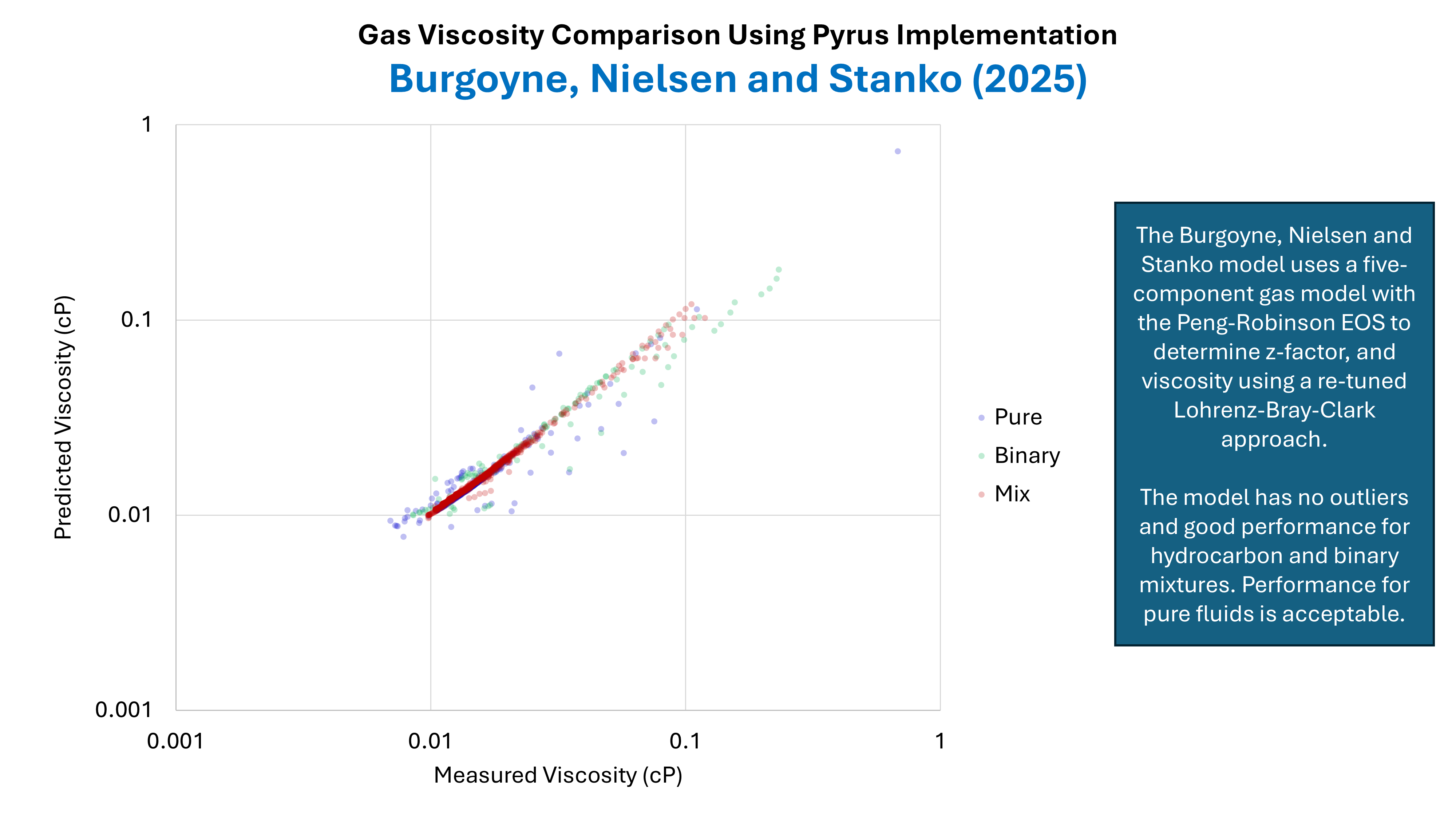
Predictive Accuracy Pure Fluids, Binary Mixtures and Hydrocarbon Mixtures
A dataset comprising 1,156 data points was compiled from published data in the literature. This dataset will be described more fully in a future blog post. The dataset contains pure fluids, binary mixtures and hydrocarbon mixtures. The predicted viscosities versus the measured viscosities for BNS are shown in Figure 3. This shows reasonably good performance for hydrocarbon fluids, with slight scatter for binary mixtures and pure fluids. Compared to some other viscosity methods (not shown) the BNS method does not appear to contain any outliers that can sometimes occur with unusual fluids. Note that the apparent poorer predictive quality for hydrocarbon mixtures near to 0.1 cP is related to the very high pressures associated with these data points which is in excess of 15,000 psia.
Python versus Java Performance
The open source code for the BNS method is implemented in Python and [Visual Basic]. As of the date of this blog post (early April 2026) it is understood that Mark Burgoyne is implementing various methods for PyResToolbox in the Rust language which should be much faster.
A comparison between the Python implementation in PyResToolbox and the Java implementation in Pyrus will be included in this blog post once completed.
References
- Burgoyne, M. W., Nielsen, M. H., and Stanko, M. 2025. A Universal, EOS-Based Correlation for Z-Factor, Viscosity and Enthalpy for Hydrocarbon and H2, N2, CO2, H2S Gas Mixtures. Paper presented at the ADIPEC, Abu Dhabi, UAE, 3-6 November. SPE-229932-MS. https://doi.org/10.2118/229932-MS.
- Herning, F. and Zipperer, L. 1936. Beitrag zur Berechnung der Zähigkeit Technischer Gasgemische aus den Zähigkeitswerten der Einzelbestandteile (Calculation of the Viscosity of Technical Gas Mixtures from Viscosity of the individual Gases), Gas und Wasserfach 79: 49–54, 69-73.
- Jossi, J. A., Stiel, L. I., and Thodos, G. 1962. The Viscosity of Pure Substances in the Dense Gaseous and Liquid Phases. AIChE Journal 8: 59-63. https://doi.org/10.1002/aic.690080116.
- Lee, A. L., Gonzalez, M. H., and Eakin, B. E. 1966. The Viscosity of Natural Gas. J Pet Technol 18 (8): 997-1000. SPE-1340-PA. https://doi.org/10.2118/1340-PA.
- Lohrenz, J., Bray, B.G., and Clark, C.R. 1964. Calculating Viscosities of Reservoir Fluids From Their Compositions. J Pet Technol 16 (10): 1171–1176. SPE-915-PA. https://doi.org/10.2118/915-PA.
- Peng, D. Y. and Robinson, D. B. 1976. A New Two-Constant Equation of State. Ind Eng Chem Fundamen 15 (1): 59-64. https://doi.org/10.1021/i160057a011.