Rather than using an empirical correlation based on a large dataset to predict fluid viscosity, the alternative is to eschew the measured data and revert to theory. Through consideration of first principles, is it possible to model how the molecules in a fluid interact, and from this ascertain the viscosity of the fluid?
The answer is that it is possible, and indeed we get to stand on the shoulders of giants such as Maxwell and Boltzmann who were the pioneers in solving the equations that govern the interactions between molecules though statistical techniques. I must confess that I haven’t delved deep into the mathematics and satisfied myself that the equations are correct (which I often do). In this case I’m happy to jump in at a level where others have used those equations to derive practical applications. One such application is the prediction of transport properties, including viscosity, that arise from these equations, as exemplified by the Chapman-Enskog theory.
Chapman-Enskog Theory
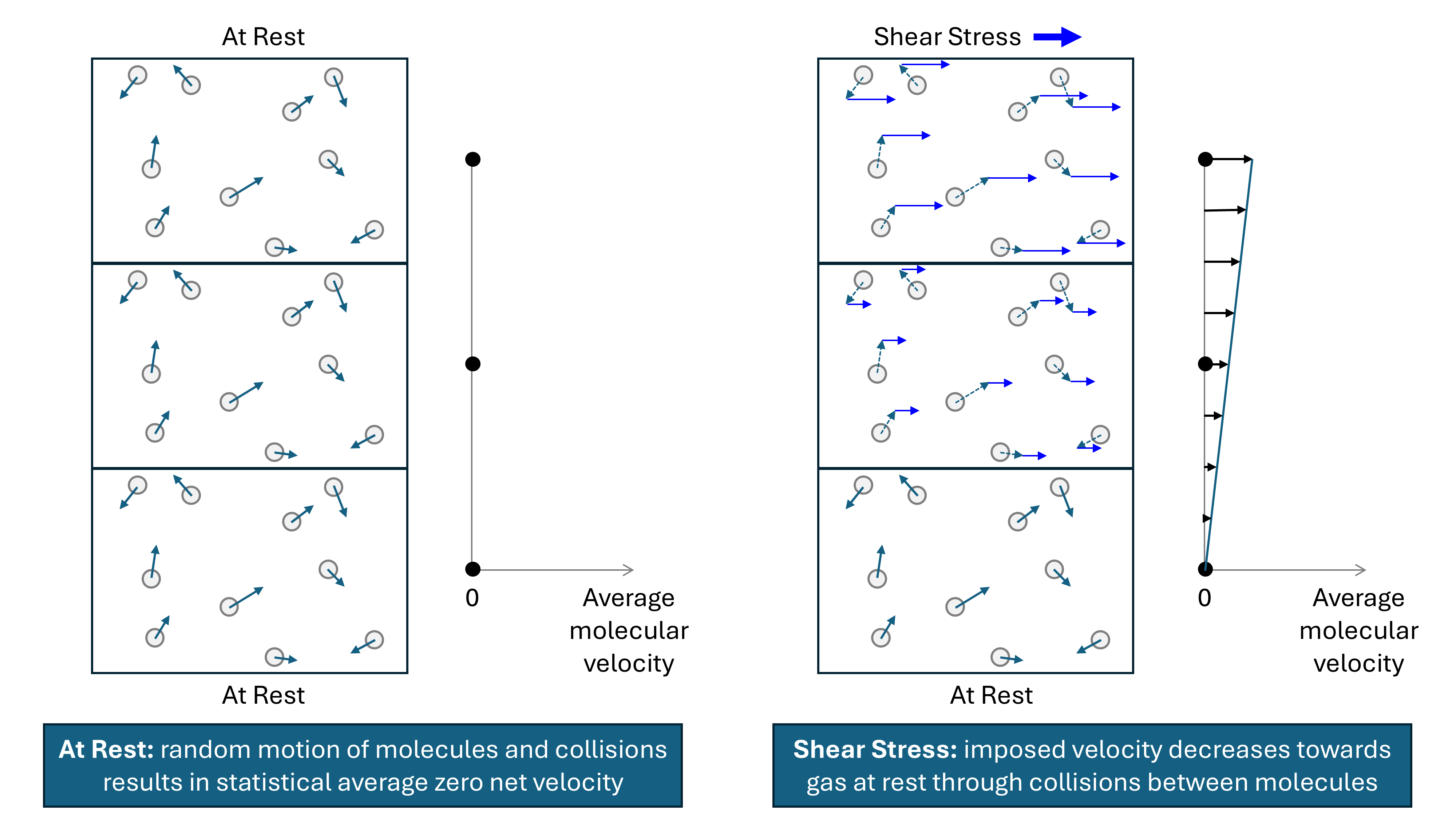
As viscosity is the measure of internal fluid friction, it follows that the application of a shear stress on part of a fluid will impart a localised velocity to that part of the fluid. We can visualise a fluid as being made up of very small elements. Elements adjacent to the moving part of the fluid will have a frictional drag imparted onto them, causing them to move with a velocity that is lower than the element imparting the frictional drag. As the distance from the element onto which the original shear stress is imparted increases, the velocity decreases, leading to a velocity gradient.
Kinetic theory models gases as molecules moving in random directions. A gas at rest can be considered to comprise a large number of molecules that are all in motion, yet with the net aggregate velocity of all molecules being zero. Within the gas molecules collide with each other, transferring momentum, and the impact of molecules on a surface leads to pressure. If molecules are contained within a smaller volume, then the number of collisions per unit surface area increases, thus leading to an increase in pressure. Temperature is related to the average kinetic energy of all the molecules. As the temperature increases, so does the average kinetic energy per molecule. For a constant pressure, the increase in temperature means that the gas expands, thus maintaining the same average kinetic energy imparted onto a unit surface area. The kinetic theory model explains the fundamental reason for the relationship between pressure, volume and temperature (PVT) of a fluid.
The mechanism for gas viscosity is related to the interaction of these randomly moving molecules within a gas. The velocity of molecules within a finite element containing gas with a bulk velocity comprises the random velocities of the molecules when the fluid is at rest, plus the bulk velocity vector. The resulting interaction between these molecules within a layer that is in motion upon the molecules of a gas that is relatively at rest, is to impose a net shear force. In principle, if all the molecular movements of individual molecules in a gas could be faithfully modelled, it is possible to calculate the aggregate properties of the gas. Thus, for a gas at a given temperature and pressure and with known molecular velocities and collisions at rest, the change in velocities arising from collisions between molecules in two adjacent layers, one at rest and the other with an imposed velocity, could be calculated. In practice, the magnitude of this net shear force can be calculated based on the theory of statistical mechanics. Statistical mechanics applies probability theory to determine the aggregate properties that arise from the interactions between large numbers of gas molecules.
In addition to the elastic collisions between molecules, the inter-molecular forces (either attractive or repulsive) can also be considered.
An illustration of how a shear force applied to a finite volume containing randomly moving molecules of gas sets up a velocity gradient via the interaction between molecules in layers of constant velocity is shown in the figure below.
It was Maxwell (1860) who first derived a probability distribution to describe molecular velocities. Boltzmann’s equation builds on this to describe the non-equilibrium behaviour of a gas and can be used to determine how macroscopic physical quantities of a gas, such as temperature and momentum, change when a gas is in motion. From this equation it is possible to derive equations that describe transport coefficients such as viscosity in terms of molecular parameters.
Solving for viscosity by considering collisions between molecules that are assumed to be rigid non-attractive spheres produces:
\[\mu=\frac{26.69(MT)^{1/2}}{\sigma^2} \label{eq:rigid_sphere}\]Where:
- μ = gas viscosity (µP)
- M = molecular weight (g/mol)
- T = temperature (K)
- σ = hard-sphere diameter (Å)
In addition to the collisions we should consider the attractive or repulsive forces between the molecules as they randomly move within the gas. One approach is known as Chapman-Enskog theory (Chapman and Cowling, 1970). This models the intermolecular interactions as being governed by an intermolecular potential energy function ψ(r) This allows the transport properties to be described through a series of integral relationships. Although the solution of the integrals requires numerical techniques, a first-order solution for viscosity is written as:
\[\mu=\frac{26.69(MT)^{1/2}}{\sigma^2\Omega_v} \label{eq:chapman_enskog}\]Where:
- μ = gas viscosity (µP)
- M = molecular weight (g/mol)
- T = temperature (K)
- σ = hard-sphere diameter (Å)
- Ωv = viscosity collision integral
Note that if there is no attraction or repulsion between molecules (collisions only) then Ωv is unity and equation \(\ref{eq:chapman_enskog}\) reduces to equation \(\ref{eq:rigid_sphere}\).
Solving the collision integral requires that a dimensionless temperature T* is found and defined as T* = kT / ε where k is the Boltzmann constant and ε is the minimum of the pair-potential energy. Lennard-Jones (1931) was the first method proposed and is frequently used. This defines the potential energy function as:
\[\psi(r)=4\varepsilon\left[\left(\frac{\sigma}{r}\right)^{12}-\left(\frac{\sigma}{r}\right)^6\right]\]The hard sphere diameter σ is determined as the value of r that causes ψ(r) to be zero. This means that there is a relationship between ε/k and σ. For example n-butane values of ε/k = 513.4 K and σ = 4.730 Å (Svehla, 1962), and ε/k = 208 K and σ = 5.869 Å (Flynn and Thodos, 1962) are both recommended in the literature, and both yield very similar values of viscosity when using equation \(\ref{eq:chapman_enskog}\).
A comparison between these two different methods is taken from Poling et al (2004) and compared in Figure 2 below. Superimposed on the Poling plot are the predicted values using the method of Chung et al (1988), and the equivalent values of ε/k and σ are also compared against those from Flynn and Thodos, and Svehla. It can be seen that despite the wide range of values for ε/k and σ, the predicted viscosities are all very close to the measured data.
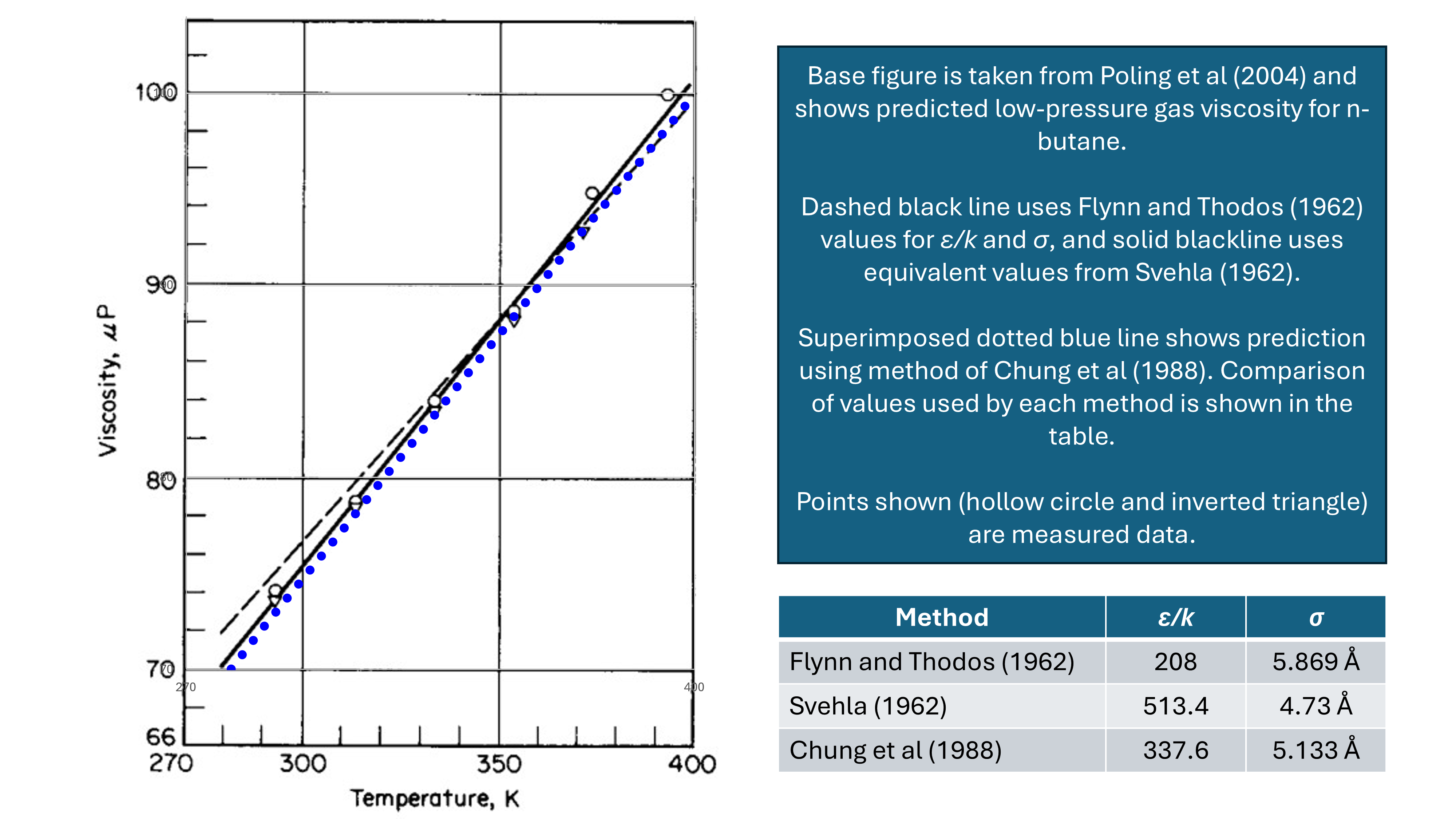
It turns out that there is no unique combination of ε/k and σ and it is difficult to derive these from experimental data. Multiple values have been proposed by different authors, all of which produce very similar viscosity results.
Chung Method
One possible solution to the Chapman-Enskog equation for low pressure gases was proposed by Chung (1988). The method here largely follows that described by Poling et al (2004).
First we must define the relationship between ε/k and σ:
\[\frac{\varepsilon}{k}=\frac{T_c}{1.2593}\] \[\sigma=0.809V_c^{1/3} \label{eq:chung_hard_sphere_definition}\]Where:
- Tc = critical temperature (K)
- Vc = critical volume (cm3/mol)
This allows the Chapman-Enskog equation to be expressed as:
\[\mu=F_c\frac{40.785(MT)^{1/2}}{V_c^{2/3}\Omega_v} \label{eq:chung_mu}\]With:
\[\Omega_v=1.16145{T^*}^{-0.14874}+0.52487\left[e^{-0.7732{T^*}}\right]+2.16178\left[e^{-2.43787{T^*}}\right]\\ -6.435\times10^{-4}{T^*}^{0.14874}\sin\left(18.0323{T^*}^{-0.7683}-7.27371\right)\] \[{T^*}=1.2593T_r \label{eq:chung_tstar}\] \[F_c=1-0.2756\omega+0.059035\mu_r^4+\kappa \label{eq:chung_fc}\]Where:
- Tr = reduced temperature [temperature / critical temperature] (dimensionless)
- ω = acentric factor (dimensionless)
- μr = dipole moment (dimensionless)
- κ = polar association factor (dimensionless)
The dipole moment and polar association factor are required for polar compounds, and are related to the irregular distibution of positive and negative charge that cause a molecular structure to act something like a mini-magnet (although the field generated is electic, not magnetic). Generally hydrocarbons are non-polar, but for mixtures containing water, it will be necessary to use the appropriate values for water. The dipole moment is related to the dielectric constant and the polarizability, and the dielectric constant is in turn related to the refractive index (Altschuller, 1953). A more in depth examination of the subject is beyond the scope of this blog post. It is sufficient to note that for common hydrocarbon compounds (C7 and smaller) experimentally measured dipole moments are available. The polar association factor is usually set to zero for hydrocarbons.
The reduced dipole moment can be calculated using:
\[\mu_r=131.3\frac{\mu}{(V_cT_c)^{1/2}} \label{eq:chung_reduced_dipole}\]For high pressure gases a different equation must be used. The low-pressure gas equation is modified through empirical correction factors to account for the higher density as pressure increases:
\[\mu=\mu^*\frac{36.344(MT_c)^{1/2}}{V_c^{2/3}} \label{eq:chung_mu_highp}\]With:
\[\mu^*=\frac{(T^*)^{1/2}}{\Omega_v}\left\{F_c\left[\frac{1}{G_2}+{E_6}y\right]\right\}+\mu^{**}\] \[G_2=\frac{E_1\left[\left(1-e^{-E_4y}\right)/y\right]+E_2G_1e^{E_5y}+E_3G_1}{E_1E_4+E_2+E_3}\] \[G_1=\frac{1-0.5y}{(1-y)^3}\] \[y=\frac{\rho{V_c}}{6}\] \[\mu^{**}=E_7y^2G_2e^{[E_8+E_9(T^*)^{-1}+E_{10}(T^*)^{-2}]}\]Where:
- Fc = molecular shape and polarity factor as per equation \(\ref{eq:chung_fc}\)
- T* = dimensionless temperature as per equation \(\ref{eq:chung_tstar}\)
- Ei = \(a_i+b_i\omega+c_i\mu_r^4+d_i\kappa\)
The coefficients for Ei are given in the table below:
| i | ai | bi | ci | di |
|---|---|---|---|---|
| 1 | 6.42302 | 50.4119 | -51.6801 | 1189.02 |
| 2 | 0.12102 × 10⁻² | -0.11536 × 10⁻² | -0.62571 × 10⁻² | 0.037283 |
| 3 | 5.28346 | 254.209 | -168.481 | 3898.27 |
| 4 | 6.62263 | 38.0957 | -8.46414 | 31.4178 |
| 5 | 19.7454 | 7.63034 | -14.3544 | 31.5267 |
| 6 | -1.89992 | -12.5367 | 4.98529 | -18.1507 |
| 7 | 24.2745 | 3.44945 | -11.2913 | 69.3466 |
| 8 | 0.79716 | 1.11764 | 0.012348 | -4.11661 |
| 9 | -0.23816 | 0.067695 | -0.8163 | 4.02528 |
| 10 | 0.068629 | 0.34793 | 0.59256 | -0.72663 |
For mixtures we must use mixing rules to determine properties of an equivalent single component fluid which is then applied to equation \(\ref{eq:chung_mu}\) or equation \(\ref{eq:chung_mu_highp}\). The mixture properties required are Tcm, Vcm, ωm, Mm, μm, and κm. These mixture properties can then be applied:
\[T_{cm}=1.2593{\left(\frac{\varepsilon}{k}\right)}_m\] \[V_{cm}=\left(\frac{\sigma_m}{0.809}\right)^3\] \[\omega_m=\frac{\sum_{i=1}^{n}\sum_{j=1}^{n}y_{i}y_{j}\omega_{ij}\sigma_{ij}^3}{\sigma_m^3}\] \[M_m=\left[\frac{\sum_{i=1}^{n}\sum_{j=1}^{n}y_{i}y_{j}\left(\varepsilon_{ij}/k\right)\sigma_{ij}^2M_{ij}^{1/2}}{\left(\varepsilon/k\right)_m\sigma_m^2}\right]^2\] \[\mu_m^4=\sigma_m^3\sum_{i=1}^{n}\sum_{j=1}^{n}\left(\frac{y_iy_j\mu_i^2\mu_j^2}{\sigma_{ij}^3}\right)\] \[\kappa_m=\sum_{i=1}^{n}\sum_{j=1}^{n}y_iy_j\kappa_{ij}\]With:
\[{\left(\frac{\varepsilon}{k}\right)}_m=\frac{\sum_{i=1}^{n}\sum_{j=1}^{n}y_{i}y_{j}\left(\varepsilon_{ij}/k\right)\sigma_{ij}^3}{\sigma_m^3}\] \[\sigma_m^3=\sum_{i=1}^{n}\sum_{j=1}^{n}y_iy_j\sigma_{ij}^3\]We also define Fcm as the mixture molecular shape and polarity factor as per equation \(\ref{eq:chung_fc}\) as:
\[F_{cm}=1-0.2756\omega_m+0.059035\mu_{rm}^4+\kappa_m \label{eq:chung_fcm}\]With:
\[\mu_{rm}=\frac{131.1\mu_m}{\left(V_{cm}T_{cm}\right)^{1/2}}\]The binary parameters are calculated using the following combining rules:
\[\sigma_{ii}=\sigma_i=0.809V_{ci}^{1/3}\] \[\sigma_{ij}=\xi_{ij}{\left(\sigma_i\sigma_j\right)}^{1/2}\] \[\frac{\varepsilon_{ii}}{k}=\frac{\varepsilon_i}{k}=\frac{T_{ci}}{1.2593}\] \[\frac{\varepsilon_{ij}}{k}=\zeta_{ij}{\left(\frac{\varepsilon_i}{k}\frac{\varepsilon_j}{k}\right)}^{1/2}\] \[\omega_{ii}=\omega_i\] \[\omega_{ij}=\frac{\omega_i+\omega_j}{2}\] \[\kappa_{ii}=\kappa_i\] \[\kappa_{ij}={\left(\kappa_i\kappa_j\right)}^{1/2}\] \[M_{ij}=\frac{2M_iM_j}{M_i+M_j}\]The Chung approach is universal for all gas conditions (temperature and pressure) and fluid types which makes it a compelling viscosity model to consider for use with Pyrus. It is also noted that at low densities, y approaches zero and G1 and G2 approach unity, thus reducing equation \(\ref{eq:chung_mu_highp}\) to equation \(\ref{eq:chung_mu}\).
Brulé-Starling Method
A similar approach to Chung was outlined by Brulé and Starling (1984) that implements Chapman-Enskog using a very similar procedure, but with a different set of coefficients and equation for E1 to E10.
The coefficients for Ei using equation \(E_i=a_i+b_i\gamma\) are given in the table below:
| i | ai | bi |
|---|---|---|
| 1 | 17.4499 | 34.0631 |
| 2 | -9.61125 × 10⁻⁴ | 7.23459 × 10⁻³ |
| 3 | 51.0431 | 169.46 |
| 4 | -0.605917 | 71.1743 |
| 5 | 21.3818 | -2.11014 |
| 6 | 4.66798 | -39.9408 |
| 7 | 3.76241 | 56.6234 |
| 8 | 1.00377 | 3.13962 |
| 9 | -7.77423 × 10⁻² | -3.58446 |
| 10 | 0.317523 | 1.15995 |
Note that the revised equation uses an orientation parameter γ. Various orientation parameters obtained by regression analysis of vapour pressure data are tabulated in the Brulé and Starling paper. It is noted by Poling et al (2004) that the Brulé and Starling method is more applicable to heavy hydrocarbons, and that if an orientation factor is not available, then the acentric factor can be used instead. Note that no mixing rules are given in the paper for mixtures. A similar mixing rule to that used for the mixture acentric factor might be considered appropriate.
Implementation in Java
The Pyrus implementation of the Chung method is shown below. Note that Pyrus uses javax.measure units and measurements with custom oilfield units. The use of these methods should be self-explanatory for anyone trying to follow the code. The code also has a number of methods to obtain component parameters such as critical properties etc. These methods are not shown and it can be assumed that the values provided are consistent with standard data reference tables.
/**
 * Gas viscosities for pure components and mixtures, both at atmospheric pressure and dense conditions. This uses
 * the first-order Chapman-Enskog viscosity equation.
 *
 * @param p mixture pressure
 * @param t mixture temperature
 * @return viscosity of the mixture
 */
protected Amount<DynamicViscosity> getViscosityChapmanEnskog(Amount<Pressure> p, Amount<Temperature> t) {
    double sigma_mix_cubed = 0.0, epsilon_over_k_mix = 0.0, mw_mix = 0.0, w_mix = 0.0, dipole = 0.0, k_mix = 0.0;
    for (FluidComponent fc_i : eos_composition.keySet()) {
        final double sigma_i = 0.809 * pow(Amount.valueOf(fc_i.v_crit() / MOLE_PER_LBMMOL, CUBIC_FOOT)
                .doubleValue(CUBIC_CENTIMETRE), 1.0 / 3.0);
        final double eta_i_over_k = Amount.valueOf(fc_i.t_crit(), RANKINE).doubleValue(KELVIN)
                / 1.2593;
        final double w_i = fc_i.acentric();
        final double k_i = ((PseudoComponent) fc_i).associationFactorChung();
        final double m_i = fc_i.mass();
        final double dipole_i = ((PseudoComponent) fc_i).dipole();
        for (FluidComponent fc_j : eos_composition.keySet()) {
            double xi_ij = 1.0; // binary interaction parameter normally set to unity
            double zeta_ij = 1.0; // binary interaction parameter normally set to unity
            double sigma_ij, eta_ij_over_k, w_ij, k_ij, m_ij;
            if (fc_i.component().equals(fc_j.component())) {
                sigma_ij = sigma_i;
                eta_ij_over_k = eta_i_over_k;
                w_ij = w_i;
                k_ij = k_i;
            } else {
                final double sigma_j = 0.809 * pow(Amount.valueOf(fc_j.v_crit() / MOLE_PER_LBMMOL, CUBIC_FOOT)
                        .doubleValue(CUBIC_CENTIMETRE), 1.0 / 3.0);
                final double eta_j_over_k = Amount.valueOf(fc_j.t_crit(), RANKINE).doubleValue(KELVIN)
                        / 1.2593;
                final double w_j = fc_j.acentric();
                final double k_j = ((PseudoComponent) fc_j).associationFactorChung();
                sigma_ij = xi_ij * sqrt(sigma_i * sigma_j);
                eta_ij_over_k = zeta_ij * sqrt(eta_i_over_k * eta_j_over_k);
                w_ij = (w_i + w_j) / 2.0;
                k_ij = sqrt(k_i * k_j);
            }
            final double m_j = fc_j.mass();
            final double dipole_j = ((PseudoComponent) fc_j).dipole();
            m_ij = (2.0 * m_i * m_j) / (m_i + m_j);
            double zi_dot_zj = eos_composition.get(fc_i) * eos_composition.get(fc_j);
            sigma_mix_cubed += zi_dot_zj * pow(sigma_ij, 3.0);
            epsilon_over_k_mix += zi_dot_zj * eta_ij_over_k * pow(sigma_ij, 3.0);
            mw_mix += zi_dot_zj * eta_ij_over_k * pow(sigma_ij, 2.0) * sqrt(m_ij);
            w_mix += (zi_dot_zj * w_ij * pow(sigma_ij, 3.0)) / sigma_mix_cubed;
            dipole += (zi_dot_zj * pow(dipole_i, 2.0) * pow(dipole_j, 2.0)) / pow(sigma_ij, 3.0);
            k_mix += zi_dot_zj * k_ij;
        }
    }
    epsilon_over_k_mix /= sigma_mix_cubed;
    double tstar_mix = t.doubleValue(KELVIN) / epsilon_over_k_mix;
    double tc_mix = 1.2593 * epsilon_over_k_mix;
    double sigma_mix = pow(sigma_mix_cubed, 1.0 / 3.0);
    double vc_mix = pow(sigma_mix / 0.809, 3.0);
    mw_mix /= epsilon_over_k_mix * pow(sigma_mix, 2.0);
    mw_mix = pow(mw_mix, 2.0);
    dipole *= sigma_mix_cubed;
    dipole = pow(dipole, 1.0 / 4.0);
    double specific_vol = mw_mix / getDensity(p, t).doubleValue(GRAM_PER_CUBIC_CENTIMETRE); // cm^3/mole
    double mu_cp = PVT.gasViscosityChung(tstar_mix, tc_mix, vc_mix, mw_mix, w_mix, k_mix, dipole,
            1.0 / specific_vol);
    }
    return Amount.valueOf(mu_cp, CENTIPOISE);
}
The method above applies the mixing rules and then calls the static PVT.gasViscosityChung method. This PVT.gasViscosityChung method is implemented as follows:
/**
 * Chung et al (1988) coefficients to calculate E_i in equations 9-6.22 and 9-6.23
 */
private static final double[] CHUNG_A = {6.42302, 0.0012102, 5.28346, 6.62263, 19.7454, -1.89992, 24.2745, 0.79716,
    -0.23816, 0.068629};
private static final double[] CHUNG_B = {50.4119, -0.0011536, 254.209, 38.0957, 7.63034, -12.5367, 3.44945, 1.11764,
    0.067695, 0.34793};
private static final double[] CHUNG_C = {-51.6801, -0.0062571, -168.481, -8.46414, -14.3544, 4.98529, -11.2913,
    0.012348, -0.8163, 0.59256};
private static final double[] CHUNG_D = {1189.02, 0.037283, 3898.27, 31.4178, 31.5267, -18.1507, 69.3466, -4.11661,
    4.02528, -0.72663};

/**
 * Component viscosity for pure gas compound following method of Chung (1984, 1988). This is based on the
 * first-order Chapman-Enskog viscosity equation which incorporates the collision diameter and the collision
 * integral.
 *
 * @param tstar dimensionless temperature (1.2593 * Tr)
 * @param tc critical temperature in Kelvin
 * @param vc critical volume in cm^3/mol
 * @param m molecular weight in g/mol
 * @param w acentric factor
 * @param k association factor correction for highly polar substances such as alcohols and acids
 * @param mu dipole moment in debye
 * @param rho density in mol/cm^3
 * @return viscosity at atmospheric pressure in cP
 */
public static double gasViscosityChung(double tstar, double tc, double vc, double m, double w, double k,
        double mu, double rho) {
    final double omega_nu = gasViscosityCollisionIntegral(tstar);
    final double mu_r = 131.3 * mu / sqrt(vc * tc);
    final double mu_rsq = mu_r * mu_r;
    final double fc = 1.0 - 0.2756 * w + 0.059035 * mu_rsq * mu_rsq + k;
    double[] e = new double[10];
    for (int i = 0; i < 10; i++) {
        e[i] = CHUNG_A[i] + CHUNG_B[i] * w + CHUNG_C[i] * mu_rsq * mu_rsq + CHUNG_D[i] * k;
    }
    double y = (rho * vc) / 6.0;
    double g1 = (1.0 - 0.5 * y) / pow(1.0 - y, 3.0);
    double g2 = (e[0] * ((1.0 - exp(-e[3] * y)) / y) + e[1] * g1 * exp(e[4] * y) + e[2] * g1)
            / (e[0] * e[3] + e[1] + e[2]);
    double mustar = sqrt(tstar) / omega_nu;
    mustar *= fc * (1.0 / g2 + e[5] * y);
    double mudblstar = e[6] * y * y * g2 * exp(e[7] + e[8] * (1.0 / tstar) + e[9] * pow(tstar, -2.0));
    mustar += mudblstar;
    final double mu_micropoise = mustar * (36.344 * sqrt(m * tc)) / pow(vc, 2.0 / 3.0);
    return mu_micropoise / 10000.0; // return in units of centiPoise
}

/**
 * Collision integral Omega_nu for Chapman-Enskog first-order viscosity equation.
 *
 * @param tstar dimensionless temperature which depends on intermolecular potential chosen
 * @return collision integral
 */
public static double gasViscosityCollisionIntegral(double tstar) {
    double omega_star = 1.16145 * pow(tstar, -0.14874) + 0.52487 * exp(-0.77320 * tstar)
            + 2.16178 * exp(-2.43787 * tstar);
    omega_star += -6.435e-04 * pow(tstar, 0.14874) * sin(18.0323 * pow(tstar, 0.7683) - 7.27371);
    return omega_star;
}
Predictive Quality
In order to test the quality of the implemented code and check the performance of the Chung method, the predicted viscosities of various fluids have been calculated and compared against measured data.
Pure Fluids
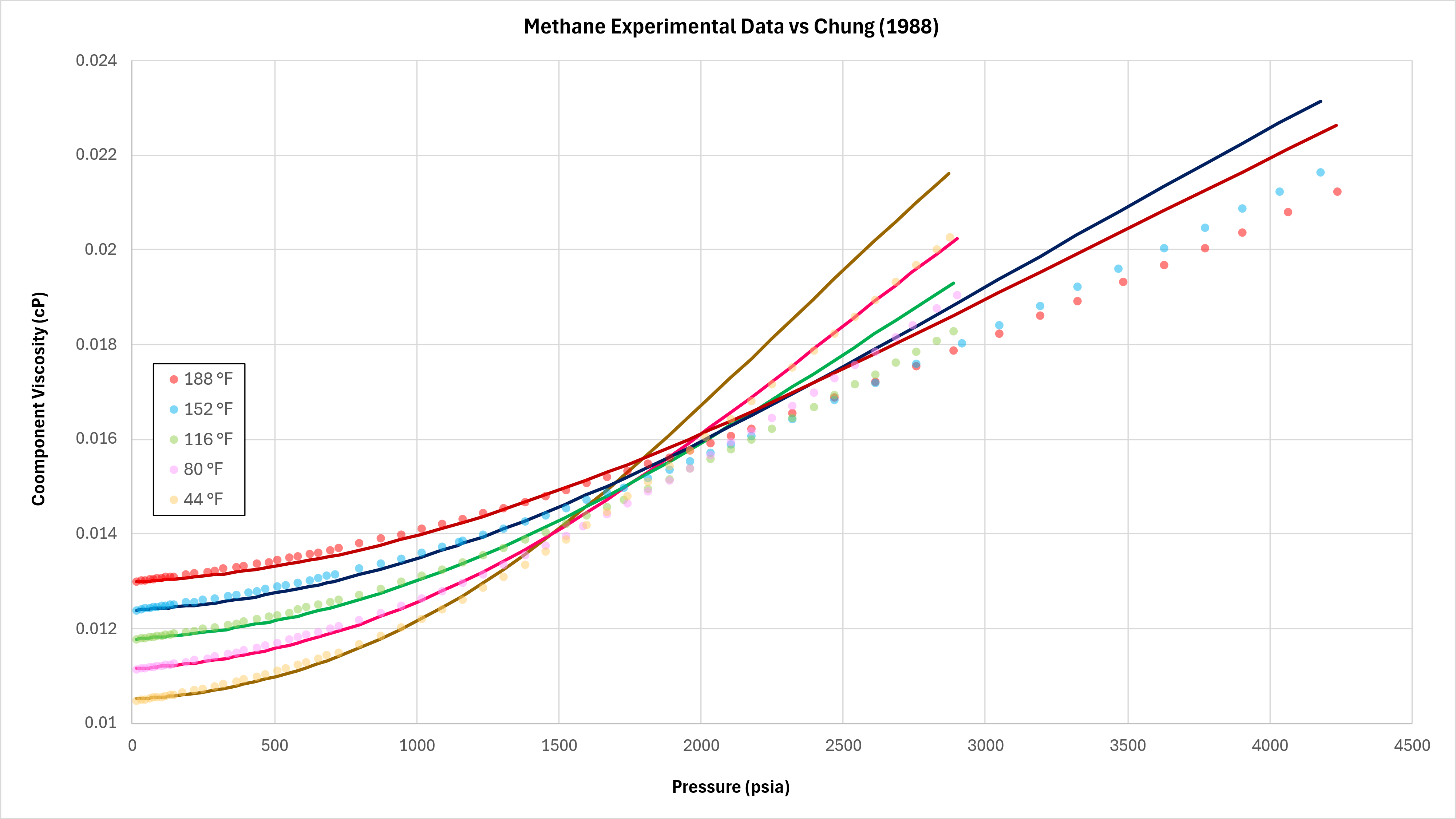
Data for methane at different temperature and pressure published by Schley et al (2004) has been compared against the implemented Chung method. This is shown in Figure 3 below.
It can be seen that the predictive quality is reasonably good at lower pressures below ~1,000 psia, but that at higher pressures the Chung method tends to overpredict the viscosity.
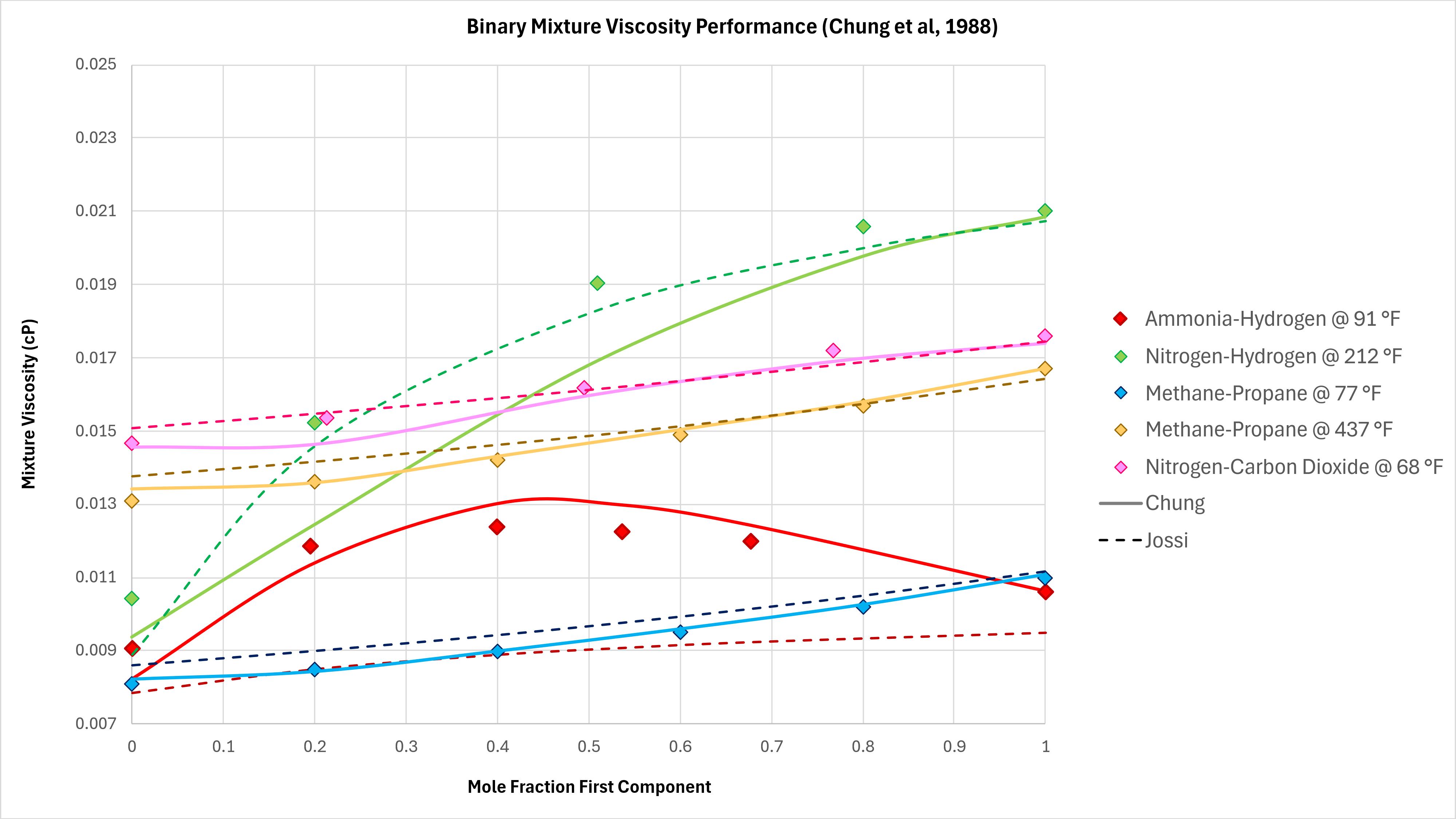
Binary Mixtures
Binary mixtures can exhibit unexpected behaviours. In moving from 100% mole fraction of one component in a binary mixture to the other, the viscosity does not always follow a monotonic trend. That is to say, the viscosity can increase and then decrease, and vice versa. Various binary mixture measured viscosity data is compared against the implemented Chung method using data taken from Poling et al (2004) as shown in Figure 4 below. All data is measured at atmospheric pressure.
The Chung method is able to capture the non-monotonic behaviour of the Ammonia-Hydrogen binary mixture, and has very good predictive capability for Methane-Propane at different temperatures. However, the predictive performance drops off for binary mixtures containing nitrogen, particular if N2 content is less than 50%.
As a comparison the Jossi, Stiel and Thodos (JST) method (as used in Lohrenz-Bray-Clark) is also shown on these charts. For binary mixtures that do not contain nitrogen, the Chung method outperforms the JST method. With binaries that contain nitrogen, this relative performance is reversed, and JST is the more accurate method.
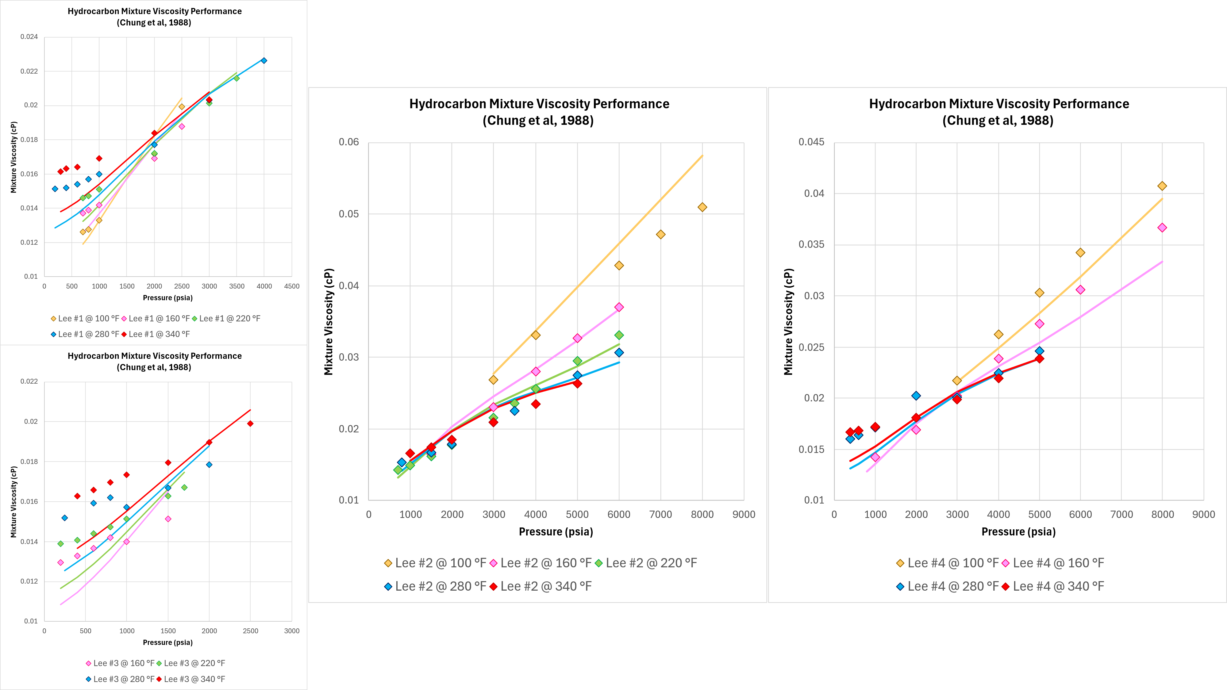
Hydrocarbon mixtures
Good performance with pure components and binary mixtures means nothing if the technique does not work on real-world fluids. Four different hydrocarbon gas mixtures and measurements of viscosity were published by Lee, Gonzalez and Eakin (1966). Whilst there are some apparent discontinuities in the measured data, this dataset is sufficient to assess the predictive performance of the implemented Chung method as shown in Figure 5 below.
It can be seen that the Chung method is able to model the correct trends in terms of the viscosity variation with temperature and pressure, and the absolute viscosity predicted is close to the measured values. However, the accuracy in some cases could be better.
References
- Altschuller, A. P. 1953. The Dipole Moments of Hydrocarbons. J Phys Chem 57 (5): 538-540. https://doi.org/10.1021/j150506a013.
- Chapman, S. and Cowling, T. G. 1970. The Mathematical Theory of Non-Uniform Gases, third edition. Cambridge: Cambridge University Press.
- Brulé, M. R. and Starling, K. E. 1984. Thermophysical Properties of Complex Systems: Applications of Multiproperty Analysis. Ind Eng Chem Process Des Dev 23 (4): 833–845. https://doi.org/10.1021/i200027a035.
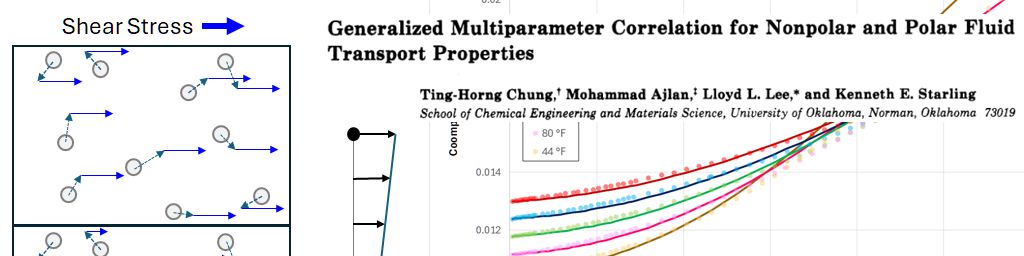
- Chung, T. H., Ajlan, M., Lee, L. L., and Starling, K. E. 1988. Generalized Multiparameter Correlation for Nonpolar and Polar Fluid Transport Properties. Ind Eng Chem Res 27: 671-679. https://doi.org/10.1021/ie00076a024.
- Flynn, L. W. and Thodos, G. 1962. Lennard-Jones Force Constants from Viscosity Data: Their Relationship to Critical Properties. AIChE J 8 (3): 362-365. https://doi.org/10.1002/aic.690080320.
- Lee, A. L., Gonzalez, M. H., and Eakin, B. E. 1966. The Viscosity of Natural Gas. J Pet Technol 18 (8): 997-1000. SPE-1340-PA. https://doi.org/10.2118/1340-PA.
- Lennard-Jones, J. E. 1931. Cohesion. Proceedings of the Physical Society 43 (5): 461–482. https://doi.org/10.1088/0959-5309/43/5/301.
- Maxwell, J. C. 1860. V. Illustrations of the Dynamical Theory of Gases. Part I. On the Motions and Collisions of Perfectly Elastic Spheres. The London, Edinburgh, and Dublin Philosophical Magazine and Journal of Science 19 (124): 19–32. https://doi.org/10.1080/14786446008642818.
- Poling, B. E., Prausnitz, J. M., and O’Connell, J. P. 2004. The Properties of Gases and Liquids, fifth edition. New York: McGraw-Hill Book Co.
- Schley, P., Jaeschke, M., Küchenmeister, C., and Vogel E. 2004. Viscosity Measurements and Predictions for Natural Gas. International Journal of Thermophysics 25 (6): 1623–1652. https://doi.org/10.1007/s10765-004-7726-5.
- Svehla, R. A. 1962. Estimated Viscosities and Thermal Conductivities of Gases at High Temperatures. Technical report, NASA-TR-R-132, National Aeronautics and Space Administration, Cleveland, Ohio (1962).