The general principle behind the Expanded Fluid (EF) model correlation is very simple: as a fluid expands there is greater distance between molecules and its fluidity increases, or rather the viscosity decreases down to a limit.
The viscosity limits are chosen as the dilute gas viscosity, the theoretical viscosity of the fluid. The form of the model is chosen deliberately so that as the density approaches zero, the viscosity approaches the gas low-pressure viscosity. Conversely, as the density approaches the compressed state density, the viscosity tends towards infinity. By comparing the density of the fluid, which effectively governs how close together its molecules are, and comparing the density to these two density endpoints, it is possible to predict viscosity.
This is a pseudo-single fluid equation, so mixing rules must be used to determine the various fitting parameters. The calculation is very sensitive to density. Any implementations using the EF model must determine an accurate liquid density to use for the calculation. based on the specific gravity which is, by definition, an exact density at a standard conditions.
Theory
Fundamentally the EF equation determines the difference in viscosity above the dilute gas viscosity. This is captured in the following equation as originally proposed by Yarranton and Satyro (2009):
\[\mu-\mu_0=c_1(exp(c_2\beta)-1)\]Where:
- μ = dynamic viscosity (cP)
- μ0 = dilute gas dynamic viscosity (cP)
- c1 = fitting parameter
- c2 = fitting parameter
With:
\[\beta=\frac{1}{\exp\left[\left(\cfrac{\rho_s^*}{\rho}\right)^n-1\right]-1}\] \[\rho_s^*=\frac{\rho_s^o}{\exp(-c_3P)}\]Where:
- ρ = density
- ρs* = density beyond which the fluid cannot be compressed without incurring a solid-liquid phase transition
- ρso = the compressed state density in a vacuum.
- n = fitting parameter
- c3 = fitting parameter
This means that the EF model requires three physical inputs, being (1) the fluid density, (2) the pressure and (3) the dilute gas viscosity. In Pyrus there are several approaches that have been coded for prediction of dilute gas viscosity, so the recommended approach of Yarranton and Satyro, to use an empirical correlation after Yaws, is not followed. In addition there are five parameters that can be varied to improve the fit to measured data. These are: ρso, n, c1, c2, and c3.
By fitting to data for n-alkanes in the NIST database, it was determined that the values for c1 and n were fixed for all hydrocarbons:
\[c_1=0.165\] \[n=0.65\]For the remaining parameters ρso, c2, and c3, these fluid-specific parameters are estimated from the physical properties of each of the components and pseudo-components. It is noted by Motahhari et al (2013) that typically Normal Boiling Point and Specific Gravity are used as these correspond to the molecular energy and size respectively. Since normal boiling point is not typically available for heavy hydrocarbons, the Molecular Weight is used as a proxy, since there are several well-known correlations that relate normal boiling point to molecular weight such as Soreide, Riazi-Daubert, Riazi-Adwani. Specific gravity is retained as the other correlating parameter.
Parameters are estimated based on a departure from a reference system based on n-paraffins. The parameter is calculated using:
\[X=X_{ref}+\Delta{X}\]Here X is either ρso or c2. The reference n-paraffin is chosen to have the same molecular mass as the hydrocarbon compound or pseudo-component of interest, and departure from paraffinic values due to aromaticity (as measured by the specific gravity relative to the molecular mass) are then determined using the following polynomial:
\[\Delta{X}=A_X\Delta{SG}^2+B_X\Delta{SG}\]With:
\[\Delta{SG}=SG-SG_{ref}\]The parameters AX and BX are fitting parameters given by:
\[A_X=b_0+\frac{b_1}{MW^{b_4}}\] \[B_X=b_2+\frac{b_3}{MW^{b_4}}\]Where the values of bn (n = 0 … 4) depend on the departure function parameter as follows:
| Property | b0 | b1 | b2 | b3 | b4 |
|---|---|---|---|---|---|
| Δρso (kg/m3) | 0 | 14640 | 739 | 0 | 0.67 |
| Δc2 | 0.4925 | -191900 | -0.371 | 83930 | 2.67 |
The n-paraffin reference values are correlated from NIST data for methane (n-C1) up to n-tetratetracontane (n-C44). This gives the following relationships:
\[SG_{ref}=a_0+\frac{a_1}{MW^{0.5}}+\frac{a_2}{MW}+\frac{a_3}{MW^2}+\frac{a_4}{MW^3}\] \[{\rho_s^o}_{ref}=\left(\frac{a_0}{MW}+a_1MW^{a_2}\right)\exp(a_3MW)+\frac{a_4}{1+a_5\exp(a_6MW)}\] \[{c_2}_{ref}=(a_0+a_1MW)\exp\left(\frac{a_2}{MW}+a_3MW\right)+a_4\ln(MW)\]Where the values of an (n = 0 … 6) depend on the departure function parameter as follows:
| Property | a0 | a1 | a2 | a3 | a4 | a5 | a6 |
|---|---|---|---|---|---|---|---|
| SG | 0.843593 | 0.1419 | -16.6 | -41.27 | 2535 | ||
| Δρso (kg/m3) | -4775 | 3.984 | 0.4 | -1.298×10⁻³ | 938.3 | 8.419×10⁻² | -1.06×10⁻³ |
| Δc2 | 9.353×10⁻² | 4.42×10⁻⁴ | -333.4 | -1.66×10⁻⁴ | 4.77×10⁻² |
There was insufficient high-pressure viscosity and density data available to determine a more suitable parameter c3 based on a departure function. Therefore c3 was correlated to molar mass as per the original EF model (Yarranton and Satyro, 2009) except that an improved estimation equation for this parameter was implemented as proposed in Motahhari et al (2013) as follows:
\[c_3=\frac{2.8\times10^{-7}}{1+3.23\exp(-1.54\times10^{-2}MW)}\]Where:
- MW = molar mass of the component (g/mol or lbm/lbm-mol)
This correlation approximates the original corelation and also converges to a fixed value of 2.8 × 10⁻⁷ kPa-1 for higher molecular weight hydrocarbons.
Mixture Workflow
The EF model equations are based on an assumption of a single component. For hydrocarbon mixtures it is necessary to determine what the equivalent single component properties would be for a representative pseudo-component, to which the EF model can then be applied.
It is also noted by Yarranton and Satyro that for heavy crudes the plus fraction must be extrapolated to multiple heavier hypothetical components, even in the case where assay data to C30+ is available. They propose an approach using an exponential distribution to split C30+ into heavier hypothetical components. Pyrus has implemented the gamm distribution
The method to get the EF model viscosity for a known compositional mixture is:
- Get the dilute gas viscosity using existing gas viscosity methods.
- Iterate over all EOS components to determine component parameters for the EF equation.
- Apply mixing rules to recombine parameters. First we get the weight (mass) fractions for each component and then apply the appropriate mixing rules to get \(c_{2,mix}\), \(\rho_{s,mix}^o\) and \(c_{3,mix}\). \(\rho_{s,mix}^*\) and \(\beta_{mix}\) are then calculated using these values.
- Apply expanded fluid model as a single pseudo-component for the mixture.
The mixing rules applicable for the EF model are:
\[\rho_{s,mix}^o=\left(\sum_{i=1}^{N}\sum_{j=1}^{N}\frac{w_iw_j}{2}\left(\frac{1}{\rho_{s,i}^o}+\frac{1}{\rho_{s,j}^o}\right)(1-\beta_{ij})\right)^{-1}\] \[\frac{c_{2,mix}}{\rho_{s,mix}^o}=\sum_{i=1}^{N}\sum_{j=1}^{N}\frac{w_iw_j}{2}\left(\frac{c_{2,i}}{\rho_{s,i}^o}+\frac{c_{2,j}}{\rho_{s,j}^o}\right)(1-\beta_{ij})\] \[c_{3,mix}=\left(\sum_{i=1}^{N}\frac{w_i}{c_{3,i}}\right)^{-1}\]Where:
- N = number of components in the mixture
- wi = mass (weight) fraction for component “i” in the mixture
- βij = binary interaction parameter that can be used to tune the model when experimental viscosity data from the mixture are available with default value of zero
If there is no experimental data to tune the model, then the binary interaction parameters can be determined using:
\[\begin{eqnarray} \beta_{ij} = \begin{cases} 0 & ( \Delta{SG_{norm}} \le 0.355 ) \\ 0.055-0.155\Delta{SG_{norm}} & ( \Delta{SG_{norm}} \gt 0.355 ) \end{cases} \end{eqnarray}\]With:
\[\Delta{SG_{norm}}=2\frac{|SG_2-SG_1|}{SG_2+SG_1}\]Implementation in Java
The Pyrus implementation of the EF method is shown below. Note that Pyrus uses javax.measure units and measurements with custom oilfield units. The use of these methods should be self-explanatory for anyone trying to follow the code. The code also has a number of methods to obtain component parameters such as critical properties etc. These methods are not shown and it can be assumed that the values provided are consistent with standard data reference tables.
/**
* Calculates the fluid viscosity using the expanded fluid theory of Yarranton and Satyro (2009). The principle is
* based on the empirical observation that as a fluid expands, the molecules are further apart and thus the
* viscosity decreases down to a limit at the dilute gas viscosity. Fundamentally the EF equation is:
*
* <pre>μ - μ<sub>0</sub> = c<sub>1</sub>(exp(c<sub>2</sub>Β) − 1)</pre>
*
* This is a pseudo-single fluid equation, so mixing rules must be used to determine the various fitting parameters.
*
* @param p mixture pressure
* @param t mixture temperature
* @param rho a specific measured density to use for the EF calculation
* @return viscosity of the mixture
*/
public Amount<DynamicViscosity> getViscosityExpandedFluid(Amount<Pressure> p, Amount<Temperature> t,
Amount<VolumetricDensity> rho) {
final int NCOMP = eos_composition.keySet().size();
// 1. Get the dilute gas viscosity using existing gas viscosity methods.
Amount<DynamicViscosity> mu_dilutegas = Amount.valueOf(0.0, CENTIPOISE);
Amount<Pressure> one_atm = Amount.valueOf(0.001, ATMOSPHERE);
boolean use_dilute_fallback = false;
try {
mu_dilutegas = getViscosityLucas(one_atm, t);
if (!Double.isFinite(mu_dilutegas.doubleValue(CENTIPOISE))) {
use_dilute_fallback = true;
}
} catch (Exception ex) {
use_dilute_fallback = true;
}
if (use_dilute_fallback) {
mu_dilutegas = getViscosityChungDilute(t);
}
if (mu_dilutegas.doubleValue(CENTIPOISE) < 0.0) {
mu_dilutegas = Amount.valueOf(1.0e-06, CENTIPOISE);
}
// 2. Iterate over all EOS components to determine component parameters for the EF equation.
double c1 = 0.165; // 0.165 from original 2009 paper consistent with 2013 paper for characterised oils
double[] c2inf = new double[NCOMP];
double[] k_c2 = new double[NCOMP];
double[] gamma_c2 = new double[NCOMP];
double[] c2 = new double[NCOMP];
double[] c3 = new double[NCOMP];
Amount<VolumetricDensity>[] rho_s_o = new Amount[NCOMP];
Amount<VolumetricDensity>[] rho_s_star = new Amount[NCOMP];
double[] inv_rhoso = new double[NCOMP];
double[] c2_over_rhoso = new double[NCOMP];
double[] wt_frac = new double[NCOMP]; // mass (weight) fractions for each component
int idx = 0;
component_loop:
for (FluidComponent fc : eos_composition.keySet()) {
PseudoComponent pc = (PseudoComponent) fc;
wt_frac[idx] = getWeightFraction(fc);
// Get the c2 infinite parameter for each component. For pure components these are defined. For pseudos we
// can calculate this value.
c2inf[idx] = pc.expandedFluidC2InfParameter();
k_c2[idx] = pc.expandedFluidKC2Parameter();
gamma_c2[idx] = pc.expandedFluidGammaC2Parameter();
// Now we calculate c2 and c3 for each component in the mixture. See equation 37 in "Extension of the
// Expanded Fluid Viscosity Model to Characterized Oils" for reference correlation parameter.
c2[idx] = expandedFluidC2Parameter(c2inf[idx], k_c2[idx], gamma_c2[idx], t);
c3[idx] = pc.expandedFluidC3Parameter();
// Density will vary for each component. See equation 36 in "Extension of the Expanded Fluid Viscosity Model
// to Characterized Oils" for reference compressed state density in vacuum.
rho_s_o[idx] = pc.expandedFluidCompressedDensityVacuumParameter();
inv_rhoso[idx] = 1.0 / rho_s_o[idx].doubleValue(KILOGRAM_PER_CUBIC_METRE);
c2_over_rhoso[idx] = c2[idx] / rho_s_o[idx].doubleValue(KILOGRAM_PER_CUBIC_METRE);
rho_s_star[idx] = expandedFluidCompressedDensityParameter(rho_s_o[idx], p, c3[idx]);
idx++;
}
// 3. Apply mixing rules to recombine parameters. First we get the weight (mass) fractions for each component
// and then apply the appropriate mixing rules to get c2_mix, rho_s_o_mix and c3_mix. rho_s_star_mix and
// beta_mix are then calculated using these values.
double[][] bij = new double[NCOMP][NCOMP]; // all zeros
Object[] fcs = eos_composition.keySet().toArray();
for (int i = 0; i < NCOMP; i++) {
for (int j = 0; j < NCOMP; j++) {
double[] sg = {
((PseudoComponent) fcs[i]).specificGravityWater(),
((PseudoComponent) fcs[j]).specificGravityWater()
};
double delta_sgnorm = 2.0 * (abs(sg[1] - sg[0]) / (sg[1] + sg[0]));
bij[i][j] = (delta_sgnorm <= 0.355) ? 0.0 : 0.055 - 0.155 * delta_sgnorm;
}
}
Amount<VolumetricDensity> rho_s_o_mix = Amount.valueOf(1.0 / mixDoubleSum(inv_rhoso, wt_frac, bij),
KILOGRAM_PER_CUBIC_METRE);
double c2_mix = mixDoubleSum(c2_over_rhoso, wt_frac, bij) * rho_s_o_mix.doubleValue(KILOGRAM_PER_CUBIC_METRE);
double c3_mix = 0.0;
for (idx = 0; idx < NCOMP; idx++) {
c3_mix += c3[idx] > 0.0 ? wt_frac[idx] / c3[idx] : 0.0;
}
c3_mix = 1.0 / c3_mix; // units of kPa^-1
Amount<VolumetricDensity> rho_s_star_mix = expandedFluidCompressedDensityParameter(rho_s_o_mix, p, c3_mix);
// 4. Fluid liquid phase density from combination of equation of state and the compressed density.
if (rho == null) {
boolean orig_use_split = use_split_for_eos;
this.use_split_for_eos = false; // temporarily disable use of split so density matches gamma
rho = Amount.valueOf(flash(t, p).rhol, POUND_PER_CUBIC_FOOT);
Amount<VolumetricDensity> rho_liq = MixtureUtils.getLiquidDensity(this, t, p);
if (getNumComponents() > 1) {
rho = rho_liq;
}
this.use_split_for_eos = orig_use_split;
}
double beta_mix = expandedFluidBetaParameter(rho_s_star_mix, rho);
// 5. Apply expanded fluid viscosity departure to dilute gas viscosity. Units are not specified in the paper,
// so we must assume that they are consistent with mu_dilutegas in mPa.s or cP.
Amount<DynamicViscosity> mu_depart = Amount.valueOf(c1 * (exp(c2_mix * beta_mix) - 1.0), CENTIPOISE);
return mu_dilutegas.plus(mu_depart);
}
/**
* Utility double sum for the expanded fluid mixture parameters.
*
* @param prop array of properties to be double summed
* @param w mass (weight) fractions for each component
* @param bij binary interaction parameters
* @return the double sum of the property for the mixture property
*/
private double mixDoubleSum(double[] prop, double[] w, double[][] bij) {
double sum = 0.0;
int n = prop.length;
for (int i = 0; i < n; i++) {
for (int j = 0; j < n; j++) {
double term = ((w[i] * w[j]) / 2.0) * (prop[i] + prop[j]) * (1.0 - bij[i][j]);
sum += term;
}
}
return sum;
}
/**
* Parameter c2 correlates to the viscosity at 25 °C. This is a fitting parameter. Mixing rules can be applied
* to c2 for each component in a mixture to get the pseudo-single fluid fitting parameter c2_mix.
*
* @param c2inf
* @param k_c2
* @param gamma_c2
* @param t temperature
* @return c2 fitting parameter
*/
private double expandedFluidC2Parameter(double c2inf, double k_c2, double gamma_c2, Amount<Temperature> t) {
return c2inf + k_c2 * exp(gamma_c2 * t.doubleValue(KELVIN));
}
/**
* Parameter beta.
*
* @param rho_s_star
* @param rho
* @return beta parameter for main EF equation
*/
private double expandedFluidBetaParameter(Amount<VolumetricDensity> rho_s_star, Amount<VolumetricDensity> rho) {
double n = 0.65; // 0.65 from original 2009 paper consistent with 2013 paper for characterised oils
final double rho_s_star_kgm3 = rho_s_star.doubleValue(KILOGRAM_PER_CUBIC_METRE);
final double rho_kgm3 = rho.doubleValue(KILOGRAM_PER_CUBIC_METRE);
final double rho_star_over_rho = rho_s_star_kgm3 / rho_kgm3;
return 1.0 / (exp(pow(rho_star_over_rho, n) - 1.0) - 1.0);
}
/**
* The compressed rho_s_star density.
*
* @param rho_s_o compressed state density in vacuum ρ<sub>s</sub><sup>o</sup>
* @param p pressure
* @param c3 constant related to molecular weight in kPa^-1
* @return compressed state density ρ<sub>s</sub>*
*/
private Amount<VolumetricDensity> expandedFluidCompressedDensityParameter(Amount<VolumetricDensity> rho_s_o,
Amount<Pressure> p, double c3) {
double rho_s_star = rho_s_o.doubleValue(KILOGRAM_PER_CUBIC_METRE) / exp(-c3 * p.doubleValue(KILO(PASCAL)));
return Amount.valueOf(rho_s_star, KILOGRAM_PER_CUBIC_METRE);
}
The PseudoComponent class methods are:
private EFParameterRegistry.EFParameters ef() {
	return EFParameterRegistry.get(component());
}

/**
 * Gets the c2 infinite parameter for the expanded fluid viscosity model.
 *
 * @return c2 infinite parameter
 */
public double expandedFluidC2InfParameter() {
	if (EFParameterRegistry.contains(component())) {
		return ef().c2inf();
	}
	return c2InfRef() + deltaC2Inf();
}

/**
 * Gets the K_c2 parameter for the expanded fluid viscosity model.
 *
 * @return K_c2 parameter
 */
public double expandedFluidKC2Parameter() {
	if (EFParameterRegistry.contains(component())) {
		return ef().kc2();
	}
	return 0.0;
}

/**
 * Gets the gamma_c2 parameter for the expanded fluid viscosity model.
 *
 * @return gamma_c2 parameter
 */
public double expandedFluidGammaC2Parameter() {
	if (EFParameterRegistry.contains(component())) {
		return ef().gammac2();
	}
	return 0.0;
}

/**
 * Gets the c3 parameter for the expanded fluid viscosity model.
 *
 * @return c3 parameter in kPa^-1
 */
public double expandedFluidC3Parameter() {
	if (EFParameterRegistry.contains(component())) {
		return ef().c3();
	}
	return 2.8e-07 / (1.0 + 3.23 * exp(-1.54e-02 * mass));
}

/**
 * Gets the compressed state density in vacuum for the expanded fluid viscosity model.
 *
 * @return compressed state density in vacuum in kg/m^3
 */
final public Amount<VolumetricDensity> expandedFluidCompressedDensityVacuumParameter() {
	double rho_s_zero;
	if (EFParameterRegistry.contains(component())) {
		rho_s_zero = ef().rhoszero();
	} else {
		rho_s_zero = rhoSZeroRef() + deltaRhoSZero();
	}
	return Amount.valueOf(rho_s_zero, KILOGRAM_PER_CUBIC_METRE);
}

/**
 * eq. 37:
 * <pre>c2inf_ref = (a0 + a1 * MW) * exp(a2 / MW + a3 * MW) + a4 * ln(MW)</pre>
 *
 * @return reference c2 infinite parameter
 */
private double c2InfRef() {
	double mw = mass;
	return (EF_A[2][0] + EF_A[2][1] * mw) * exp(EF_A[2][2] / mw + EF_A[2][3] * mw) + EF_A[2][4] * log(mw);
}

/**
 * eq. 36:
 * <pre>rhoso_ref = (a0 / MW + a1 * MW ^ a2) * exp(a3 * MW) + a4 / (1 + a5 * exp(a6 * MW))</pre>
 *
 * @return reference compressed density in vacuum
 */
private double rhoSZeroRef() {
	double mw = mass;
	return (EF_A[1][0] / mw + EF_A[1][1] * pow(mw, EF_A[1][2])) * exp(EF_A[1][3] * mw)
			+ EF_A[1][4] / (1.0 + EF_A[1][5] * exp(EF_A[1][6] * mw));
}

/**
 * eq. 34:
 * <pre>sg_ref = a0 + a1 / (MW ^ 0.5) + a2 / MW + a3 / (MW ^ 2) + a4 / (MW ^ 3)</pre>
 *
 * @return reference specific gravity relative to water
 */
private double sgRef() {
	double mw = mass;
	return EF_A[0][0] + EF_A[0][1] / sqrt(mw) + EF_A[0][2] / mw + EF_A[0][3] / (mw * mw)
			+ EF_A[0][4] / pow(mw, 3.0);
}

private double deltaC2Inf() {
	final double delta_c2inf = deltaX(1); // Table 4 in 2013 paper, index 1 is Delta_c2
	if (eft_debug) {
		LOG.log(Level.FINEST, "delta_c2inf: {0}", new Object[]{delta_c2inf});
	}
	return delta_c2inf;
}

private double deltaRhoSZero() {
	final double delta_rhoso = deltaX(0); // Table 4 in 2013 paper, index 0 is Delta_rho_s_zero
	if (eft_debug) {
		LOG.log(Level.FINEST, "delta_rhoso: {0}", new Object[]{delta_rhoso});
	}
	return delta_rhoso;
}

private double deltaSG() {
	final double delta_sg = gamma - sgRef();
	if (eft_debug) {
		LOG.log(Level.FINEST, "delta_sg: {0}", new Object[]{delta_sg});
	}
	return delta_sg;
}

/**
 * eq. 38:
 * <pre>Delta_x = (b0 + b1 / mw ^ b4) * Delta_SG ^ 2 + (b2 + b3 / mw ^ b4) * Delta_SG</pre>
 *
 * @return departure function from reference n-paraffin for heavy hydrocarbons
 */
private double deltaX(int prop_idx) {
	double mw = mass;
	double delta_sg = deltaSG();
	final double mw_pow_b4 = pow(mw, EF_B[prop_idx][4]);
	double delta_x = (EF_B[prop_idx][0] + EF_B[prop_idx][1] / mw_pow_b4) * delta_sg * delta_sg;
	delta_x += (EF_B[prop_idx][2] + EF_B[prop_idx][3] / mw_pow_b4) * delta_sg;
	return delta_x;
}
The EFParameterRegistry contains all the constants for the EF viscosity model.
import java.util.Collections;
import java.util.HashMap;
import java.util.Map;

/**
 * Registry of lookup values for the expanded fluid viscosity model. Values taken from "Process Simulation Using the
 * Expanded Fluid Model for Viscosity Calculations" by Loria, Motahhari, Satyro, and Yarranton (2014).
 *
 * @author Peter Kirkham
 */
public class EFParameterRegistry {

    /* == DECLARE GLOBAL VARIABLES == */
    public record EFParameters(double c2inf, double kc2, double gammac2, double rhoszero, double c3) {
    }

    /* == ENABLE LOGGING == */
    transient private static final java.util.logging.Logger LOG
            = java.util.logging.Logger.getLogger(EFParameterRegistry.class.getName());

    private static final Map<String, EFParameters> REGISTRY;

    static {
        Map<String, EFParameters> m = new HashMap<>();
        m.put("CH4", new EFParameters(0.1082, 0.0, 0.0, 549.29, 7.21e-07));
        m.put("C2H6", new EFParameters(0.1412, 0.0, 0.0, 716.44, 0.0));
        m.put("C3H8", new EFParameters(0.1684, 0.0, 0.0, 772.12, 4.94e-07));
        m.put("NC4", new EFParameters(0.1898, 0.0, 0.0, 812.05, 4.79e-07));
        m.put("NC5", new EFParameters(0.2049, 0.0, 0.0, 834.29, 8.06e-07));
        m.put("NC6", new EFParameters(0.2271, 0.0, 0.0, 869.06, 8.23e-07));
        m.put("NC7", new EFParameters(0.2013, 0.0, 0.0, 849.65, 0));
        m.put("NC8", new EFParameters(0.2275, 0.0, 0.0, 867.61, 3.88e-07));
        m.put("NC9", new EFParameters(0.2571, 0.0, 0.0, 886.29, 3.16e-07));
        m.put("NC10", new EFParameters(0.246, 0.0, 0.0, 876.53, 3.86e-07));
        m.put("NC12", new EFParameters(0.2504, 0.0, 0.0, 871.96, 3.91e-07));
        m.put("NC14", new EFParameters(0.2551, 0.0, 0.0, 870.72, 3.61e-07));
        m.put("NC16", new EFParameters(0.308, 0.0, 0.0, 890.93, 2.64e-07));
        m.put("NC20", new EFParameters(0.3572, 0.0, 0.0, 910.07, 0));
        m.put("NC24", new EFParameters(0.3376, 0.0, 0.0, 895.54, 7.45e-07));
        m.put("NC26", new EFParameters(0.3591, 0.0, 0.0, 897.3, 5.37e-05));
        m.put("3_M-C5", new EFParameters(0.2113, 0.0, 0.0, 865.58, 1.08e-06));
        m.put("2,2_DiM-C5", new EFParameters(0.1426, 0.0, 0.0, 796.41, 1.00e-06));
        m.put("2_M-C6", new EFParameters(0.2031, 0.0, 0.0, 850.07, 4.36e-06));
        m.put("2,2_DiM-C6", new EFParameters(0.1901, 0.0, 0.0, 833.69, 1.07e-05));
        m.put("2_M-C7", new EFParameters(0.2438, 0.0, 0.0, 874.39, 4.33e-05));
        m.put("Cy-C5", new EFParameters(0.2457, 0.0, 0.0, 967.86, 1.00e-07));
        m.put("Cy-C6", new EFParameters(0.2592, 0.0, 0.0, 935.28, 6.12e-07));
        m.put("Cy-C8", new EFParameters(0.2310, 0.0, 0.0, 937.84, 6.17e-06));
        m.put("C6H6", new EFParameters(0.2081, 0.0, 0.0, 1048.8, 3.81e-06));
        m.put("C7H8", new EFParameters(0.2111, 0.0, 0.0, 1050.0, 3.72e-07));
        m.put("O-X", new EFParameters(0.2289, 0.0, 0.0, 1050.4, 2.43e-07));
        m.put("P-X", new EFParameters(0.2073, 0.0, 0.0, 1030.8, 0));
        m.put("C8H10", new EFParameters(0.2787, 0.0, 0.0, 1094, 2.50e-07));
        m.put("H2O", new EFParameters(0.1912, 49.2, 0.0185, 1304.76, 1.29e-07));
        m.put("H2S", new EFParameters(0.2033, 0.0, 0.0, 1172.97, 8.81e-05));
        m.put("CO2", new EFParameters(0.2226, 0.0, 0.0, 1588.0, 2.13e-07));
        m.put("N2", new EFParameters(0.1082, 0.0, 0.0, 1006.94, 2.09e-07));
        REGISTRY = Collections.unmodifiableMap(m);
    }

    private EFParameterRegistry() {
    }

    public static EFParameters get(String name) {
        EFParameters p = REGISTRY.get(name);
        if (p == null) {
            throw new IllegalArgumentException("No EF parameters registered for component: " + name);
        }
        return p;
    }

    public static boolean contains(String name) {
        return REGISTRY.containsKey(name);
    }
}
Density Determination
The EF model was developed on the basis of measured density data. To use the EF model, it is important to have accurate, predictive density for both vapour and liquid phases. In particular, near to the compressed state density conditions, the method is very sensitive to the predicted density.
Predictive density methods include:
- Tuned volume shift: Cubic equations of state are notorious for poor volume (and hence density) predictions. Despite this, in any given cubic equation of state a volume shift can be applied to ‘correct’ the predicted volume without affecting the pressure and temperature phase equilibrium. adjusted to match measured data.
- Rackett compressibility: Based on critical properties the modified Rackett equation can be used to estimate saturated density based on the temperature, and knowledge of a component’s critical volume and temperature. It should only be used for temperatures that are well below the critical point (Tr < 0.85).
- Alani and Kennedy method: Based on the van der Waals cubic equation of state. This is an older method with limited accuracy.
- ASTM 1250-80 method: We can set one known density point based on the component specific gravity (relative density to water = 1) at standard temperature (60 °F) and then use the ASTM 1250-80 method to predict the density at a second temperature. This method is applicable to hydrocarbons, but not to other types of compounds.
The ASTM 1250-80 correlation for the thermal expansion of stable oils is given as:
\[\rho_{T_1}=\rho_{T_0}\exp\left[-A(T_1-T_0)(1+0.8A(T_1-T_0))\right]\]The bottom line is that is necessary to obtain an accurate density if the EF model is to be used. This is the greatest challenge for the technique. A deeper dive into density prediction is beyond the scope of this blog post and will be covered elsewhere.
Initial Results
Motahhari et al (2013) includes an assay for the WC-B-B2 bitumen (heavy dead oil) from western Canada. The viscosity versus pressure and temperature and density versus pressure and temperature are provided for this oil in the form of plots of experimental data against model predictions. The experimental datapoints were digitised and used to compare the results obtained using the Pyrus implementation.
These results are shown in Figure 1 below:
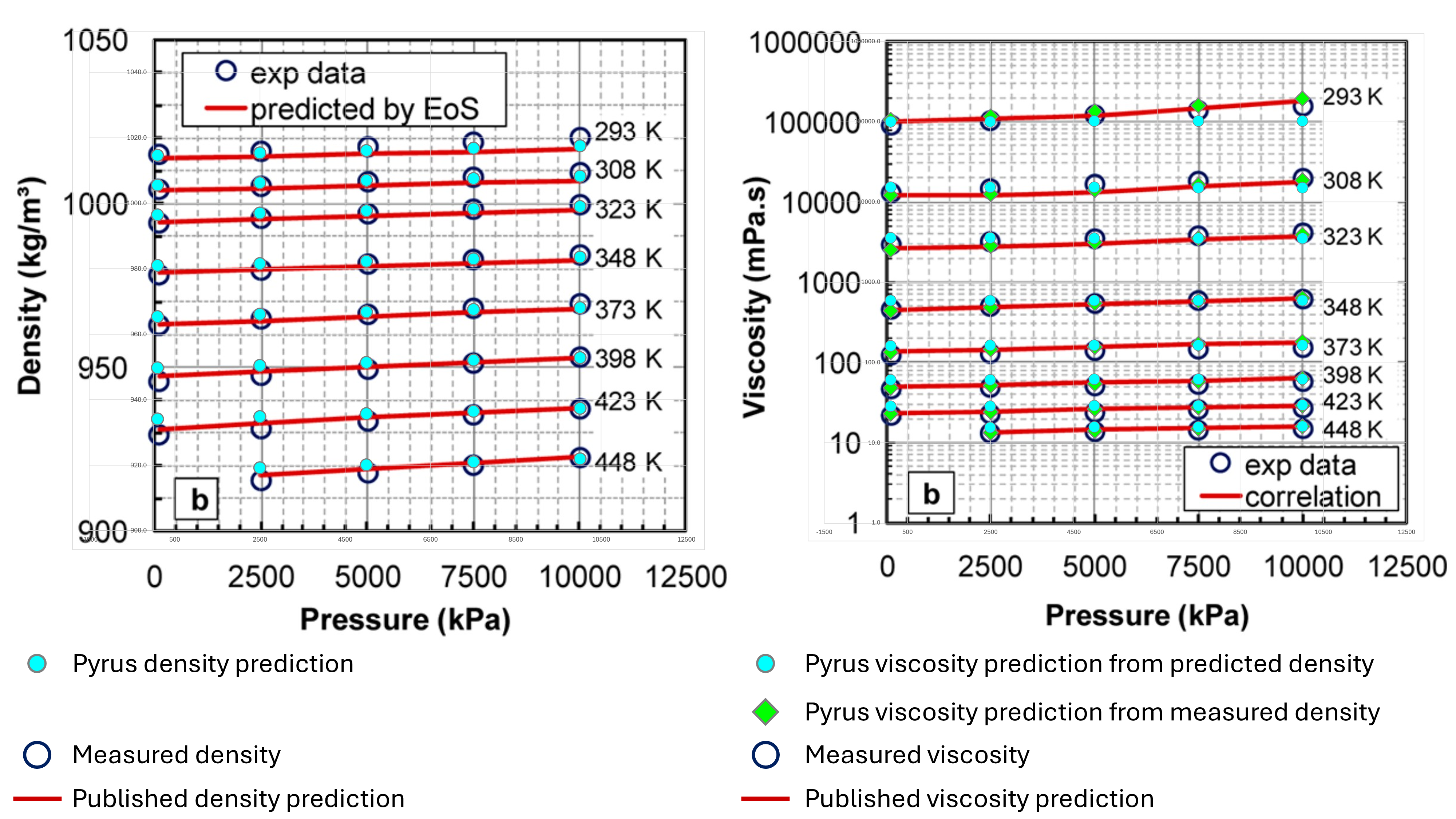
It can be seen that the prediction of viscosity using the experimental densities is reasonably close to the measured viscosity values. However, the prediction of density shows some deviations, particularly at higher pressure and lower temperature, where density is underpredicted, or at lower pressure and higher temperature, where density is overpredicted. Although the predicted density appears to be similar to the published density predictions of Motahhari et al (2013) using their equation of state, the use of these predicted densities in Pyrus leads to errors in the predicted viscosity. Although the differences do not appear large, it must be remembered that this is a logarithmic scale for the viscosity and thus the differences are quite significant in relative percentage error terms.
References
- Alani, G, H. and Kennedy, H. T. 1960. Volumes of Liquid Hydrocarbons at High Temperatures and Pressures. Pet Trans 219 (1): 288–292. https://doi.org/10.2118/1399-G.
- Loria, H., Motahhari, H., Satyro, M. A., and Yarranton, H. W. 2014. Process Simulation Using the Expanded Fluid Model for Viscosity Calculations. Chem Eng Res Des 92 (2014): 3083-3095. https://doi.org/10.1016/j.cherd.2014.06.019.
- Motahhari, H., Satyro, M. A., Taylor, S. D., and Yarranton, H. W. 2013. Extension of the Expanded Fluid Viscosity Model to Characterized Oils. Energy Fuels 27 (4): 1881-1898. https://doi.org/10.1021/ef301575n.
- Ramos-Pallares, F., Schoeggl, F. F., Taylor, S. D., Satyro, M. A., and Yarranton, H. W. 2015. Predicting the Viscosity of Hydrocarbon Mixtures and Diluted Heavy Oils Using the Expanded Fluid Model. Energy Fuels 30 (5): 3575-3595. https://doi.org/10.1021/acs.energyfuels.5b01951.
- Regueira, V. B., Pereira, V. J., Costa, G. M. N.,, and Vieira de Melo, S, A. B. 2018. Improvement of the Expanded Fluid Viscosity Model for Crude Oils: Effects of the Plus Fraction Characterization Methods and Density. Energy Fuels 32 (2): 1624–1633. https://doi.org/10.1021/acs.energyfuels.7b03735.
- Satyro, M. A. and Yarranton, H. W. 2010. Expanded Fluid-Based Viscosity Correlation for Hydrocarbons Using an Equation of State. Fluid Phase Equilib 298 (2010): 1-11. https://doi.org/10.1016/j.fluid.2010.06.023.
- Yarranton, H. W. and Satyro, M. A. 2009. Expanded Fluid-Based Viscosity Correlation for Hydrocarbons. Ind Eng Chem Res 48 (7): 3640-3648. https://doi.org/10.1021/ie801698h.