Lohrenz, Bray and Clark (1964) outlined an approach to calculating visocity of any hydrocarbon, whether gas or oil. The method first calculates a low-pressure pure component gas viscosity for all components which incorporates any effects from temperature. The component viscosities are combined into a low-pressure mixture gas viscosity using a mixing rule. Depending on whether the fluid density is gaseous or liquid, either a corresponding states approach is used for gas, or a residual viscosity approach is used for liquid.
The Lohrenz-Bray-Clark (LBC) correlation is often used in the oil and gas industry. It is incorporated into almost all software packages that deal with fluid properties, not because it is necessarily the best approach, but because it is expected that the method should be available. As such it is almost universally applied. Furthermore, it is intended to calculate the viscosity of both gases and liquids, at high and low temperature and pressure.
To add to the confusion, the LBC approach describes a workflow to determine viscosity for any hydrocarbon fluid. It builds on and incorporates existing equations, and does not introduce any new equations of its own. In particular, the residual viscosity approach to determine viscosity of liquids uses the approach of Jossi, Stiel and Thodos (1962). It was noted that this could be applied to gases as well as liquids, but the absence of a suitably accurate gas density prediction method led to their recommendation to use the older graphical corresponding states method (albeit with computer assisted lookup table interpolation).
When it is stated that the LBC co-efficients need to be tuned to match a viscosity model, what is really being stated is that the Jossi, Stiel and Thodos co-efficients need to be tuned. This is expected, as the original paper provided different co-efficients for different types of fluid.
In other words, any criticisms and shortcomings perceived of the LBC method are most likely issues related to the underlying viscosity equations being used. Lohrenz et al observe that since the calculation procedure is a sequence of steps, it is possible to update or change any step. By substituting new and improved methods into the steps, the workflow remains relevant, and its overall accuracy is improved.
Lohrenz-Bray-Clark Method
The LBC approach is based on the residual viscosity concept and the theory of corresponding states. A series of steps is followed as shown in the workflow of Figure 1. The process first determines the low-pressure gas viscosity for all composition components. From this the mixture low-pressure gas viscosity is calculated. This determines the fluid viscosity at the target temperature and low pressure. Different approaches are then used to determine the residual viscosity depending on whether the fluid is gaseous or liquid in nature. This determines the fluid viscosity at the target temperature and pressure.
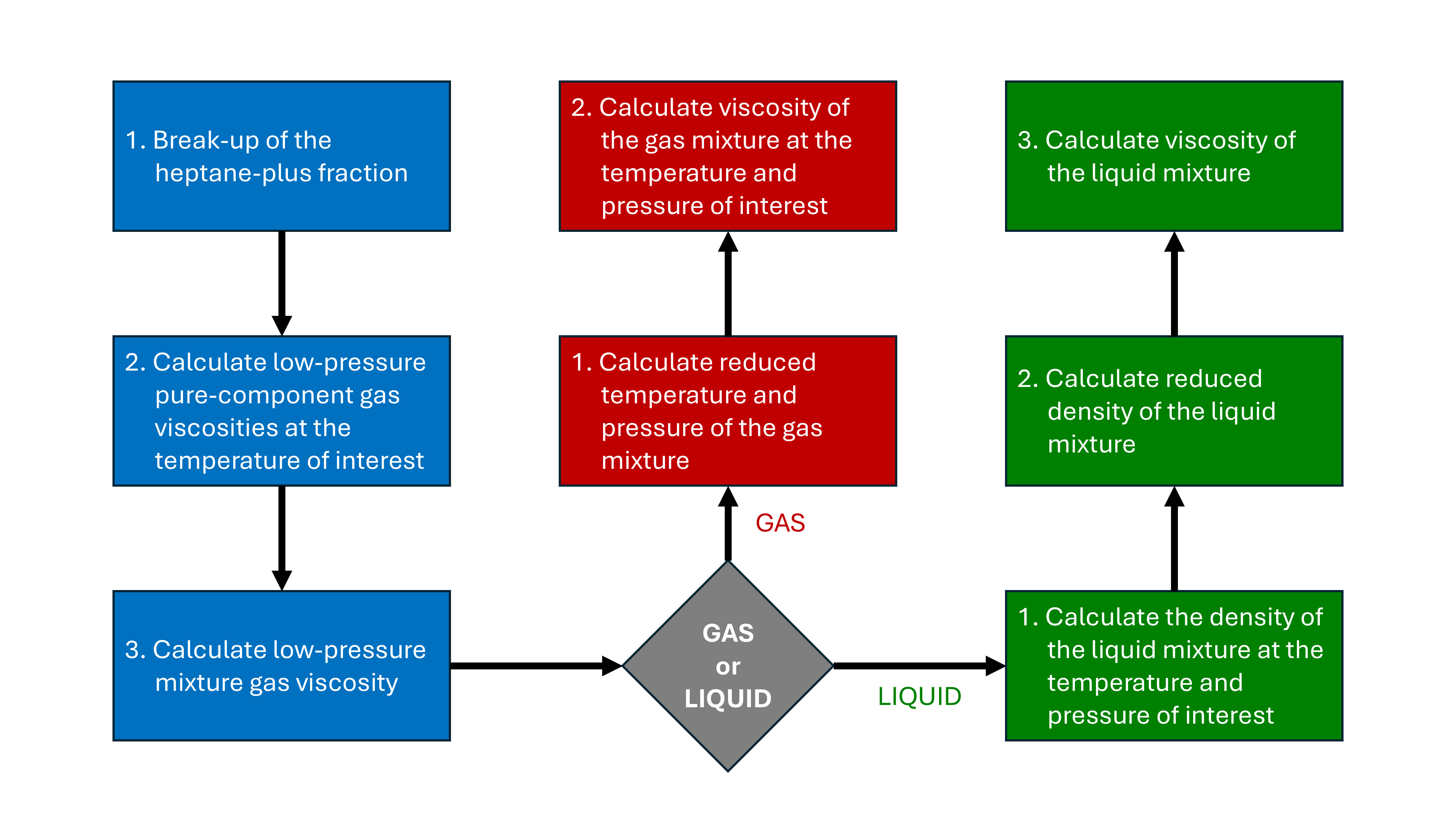
Details for each step are as follows:
-
Break-up of the heptane-plus fraction.
The C7+ fraction is ideally split into smaller components from C7 through to C40. The LBC paper notes that it is assumed that the split components are normal paraffins for convenience, and their procedure did not account for paraffinic or aromatic character in the split fractions. This shortcoming was outweighed by the observation that including even small amounts of very heavy fractions avoids large discrepancies in the results.
-
Calculate low-pressure pure-component gas viscosities at the temperature of interest.
The low-pressure pure component gas viscosity is calculated for all components in the mixture using the Stiel and Thodos correlation.
For Tri < 1.5:
\[\mu_i^{*}\xi_i=34\times10^{-5}T_{ri}^{0.94}\]For Tri > 1.5:
\[\mu_i^*\xi_i=17.78\times10^{-5}\left(4.58T_{ri}-1.67\right)^{5/8}\]With:
\[T_{ri}=\frac{T}{T_{ci}}\] \[\xi_i=\frac{T_{ci}^{1/6}}{M_{wi}^{1/2}p_{ci}^{2/3}}\]Where:
- Tri = component reduced density
- ξi = component viscosity-reducing parameter ≈ 1 / μci (cP-1)
- Tci = component critical temperature (K)
- pci = component critical pressure (atm)
- Mwi = component molecular weight (g/mol)
-
Calculate low-pressure mixture gas viscosity.
Herning and Zipperer (1936) is used as a mixing rule to combine the pure component low-pressure viscosities.
\[\mu^{*}=\frac{\sum_{i=1}^{n}\mu_i^{*}z_i\sqrt{M_i}}{\sum_{i=1}^{n}z_i\sqrt{M_i}}\]Other mixing rules were tested, and it was found that Herning and Zipperer had the best performance when tested against the available dataset.
-
Determine whether fluid is GAS or LIQUID.
No guidance is provided in the LBC paper as to how this should be determined.
If GAS fluid:
-
Calculate reduced temperature and pressure of the gas mixture.
Average pseudocritical values can be calculated using simple mixing rules for the critical properties.
\[T_r=\frac{T}{\sum_{i=1}^{n}\left(z_iT_{ci}\right)}\] \[p_r=\frac{p}{\sum_{i=1}^{n}\left(z_ip_{ci}\right)}\] -
Calculate viscosity of the gas mixture at the temperature and pressure of interest.
The chart of Baron, Roof and Wells is used which plots the viscosity ratio μ / μ* similar to Comings et al (1944). Baron, Roof and Wells contains data for several pure components at different temperatures and pressures which allows interpolation of the points to be computed. Essentially this is a lookup table approach for the graphical Comings et al approach.
\[\frac{\mu}{\mu^{*}}=f(T_r, P_r)\]
Else if LIQUID fluid:
-
Calculate the density of the liquid mixture at the temperature and pressure of interest.
The LBC paper simply states that “the Alani and Kennedy method is used”, but is light details. The equation is used without modification with the exception of nonhydrocarbon components, where new constants are used for hydrogen sulphide, nitrogen and carbon dioxide so as to improve the liquid density predictions for reservoir mixtures containing these components.
-
Calculate reduced density of the liquid mixture.
Reduced density is given by the density ρ divided by the critical density ρc.
\[\rho_r=\frac{\rho}{\rho_c}\]The pseudocritical density is calculated from the pseudocritical volume.
\[\rho_c=\frac{M_w}{V_c}\]With:
\[V_c=\sum_{\substack{i=1\\i\neq C_{7+}\\}}^{n}(z_iV_{ci})+z_{C_{7+}}V_{cC_{7+}}\] \[V_{cC_{7+}}=2.573+0.015122M_{C_{7+}}-27.6561G_{C_{7+}}+0.070615M_{C_{7+}}G_{C_{7+}}\]Where:
- Vc = critical volume
- VcC7+ = critical volume of heptane-plus fraction
- \(M_{C_{7+}}\) = molecular weight of heptane-plus fraction (lbm/lbm-mol)
- \(G_{C_{7+}}\) = specific gravity of heptane-plus fraction (water = 1.0)
-
Calculate viscosity of the liquid mixture.
The relationship developed by Jossi et al (1962) is used to determine the liquid mixture viscosity μ. Jossi, Stiel and Thodos (1962) introduced an alternative approach based on the residual viscosity. It was determined that the residual viscosity should be a function of the density and dimensional constants specific to each fluid. Through application of dimensional analysis and computer-aided polynomial regression (a novelty at that time), an analytical relationship was found:
\[\left[\left({\mu-\mu^{*}}\right)\xi+10^{-4}\right]^{1/4}=a_1+a_2\rho_r+a_3\rho_r^2+a_4\rho_r^3+a_5\rho_r^4\]With:
\[\xi=\frac{[\sum_{i=1}^{n}(z_iT_{ci})]^{1/6}}{[\sum_{i=1}^{n}(z_iM_{i})]^{1/2}[\sum_{i=1}^{n}(z_iP_{ci})]^{2/3}}\]Where:
- μ* = low-pressure mixture gas viscosity (cP)
- (μ − μ*) = residual viscosity (cP)
- ξ = mixture viscosity-reducing parameter ≈ 1 / μc (cP-1)
It is noted that this relationship holds for most fluids where critical compressibility was between 0.269 to 0.294. These fluids include argon, nitrogen, oxygen, carbon dioxide, sulphur dioxide, methane, ethane, propane, i-butane, n-butane, and n-pentane. Fluids with critical compressibilities outside of this range (hydrogen, water and ammonia) exhibited similar trends, but with deviation from the principal trend in the lower density region (Pr < 1.0). The coefficients for the different fluids are:
Parameter Normal Fluids Hydrogen Ammonia Water zc 0.269 to 0.294 0.305 0.242 0.231 a1 0.10230 0.10616 0.10670 0.10721 a2 0.023364 -0.042426 0.022655 0.040646 a3 0.058533 0.17553 0.035749 0.0026282 a4 -0.040758 -0.12295 -0.032153 -0.0054430 a5 0.0093324 0.028149 0.0089998 0.0017979 The Jossi et al residual viscosity could also be described as a corresponding states approach since it is based on a reduced increase in viscosity above the dilute gas viscosity in terms of the reduced density, and this is similar for many fluids. Here we distinguish between methods that model the viscosity ratio, μ / μ* = f(Tr , pr), as corresponding states models, and those that model the additional viscosity, μ = μ* + f(Tr , pr), as residual viscosity models.
Lohrenz, Bray and Clark note that because the calculation procedure is a sequence of steps, it is possible to update or change any step. They note that since they devised the procedure, new techniques had emerged which could both simplify the calculations and/or improve the accuracy. It is also noted that it should be possible to make gas viscosity predictions using an identical procedure to that applied for liquid viscosities, but the lack of a reliable gas density prediction method (at the time the LBC paper was written) prevented them from pursuing this route.
Implementation in Java
The Pyrus implementation of the Lohrenz-Bray-Clark method is shown below. Note that Pyrus uses javax.measure units and measurements with custom oilfield units. The use of these methods should be self-explanatory for anyone trying to follow the code.
/**
 * Implements the Lohrenz-Bray-Clark viscosity procedure in accordance with the outline proposed in their 1964
 * paper.
 *
 * @param p mixture pressure
 * @param t mixture temperature
 * @return viscosity of the mixture
 */
public Amount<DynamicViscosity> getViscosityLBC(Amount<Pressure> p, Amount<Temperature> t) {

    // Generate dilute gas viscosities for the mixture.
    FastMap<FluidComponent, Amount<DynamicViscosity>> xi_mui = new FastMap<>(eos_composition.size());
    StringBuilder sb = null;
    for (FluidComponent fc : eos_composition.keySet()) {
        Condition critical_pt = fc.criticalPoint();
        final Double zi = eos_composition.get(fc);
        final double mplus = fc.mass();
        final double tc_degk = critical_pt.getTemperature().doubleValue(KELVIN);
        final double tri = t.doubleValue(KELVIN) / tc_degk;
        final double pc_atm = critical_pt.getPressure().doubleValue(ATMOSPHERE);
        final double xi = PVT.viscosityReducingParameter(tc_degk, pc_atm, mplus);
        final double mui_cp = PVT.gasViscosityLowPressureStielThodos(tri, xi);
        xi_mui.put(fc, Amount.valueOf(mui_cp, CENTIPOISE));
    }

    // Apply Herning and Zipperer (1936) mixing rule to get mixture dilute gas viscosity.
    Amount<DynamicViscosity> mu_star = mixingRuleHerningZipperer(xi_mui, eos_composition);

    // Calculate density
    double rho = getDensity(p, t).doubleValue(POUND_PER_CUBIC_FOOT);

    // Calculate reduced density
    double vcrit = 0.0;
    for (FluidComponent fc : eos_composition.keySet()) {
        final double vci = eos_composition.get(fc) * fc.criticalPoint().getVolume().doubleValue(CUBIC_FOOT);
        vcrit += vci;
    }
    double molw = getMolecularMass();
    double rho_c = molw / vcrit; // lbm/ft^3
    double rho_r = rho / rho_c;

    // Jossi et al polynomial
    double tc_degk = criticalTemperatureEstimate().doubleValue(KELVIN);
    double pc_atm = criticalPressureEstimate().doubleValue(ATMOSPHERE);
    double xi = PVT.viscosityReducingParameter(tc_degk, pc_atm, molw);
    double mu = PVT.viscosityJossiStielThodos(rho_r, xi, mu_star.doubleValue(CENTIPOISE));
    return Amount.valueOf(mu, CENTIPOISE);
}

/**
 * In a simplification of the kinetic theory approach, ignoring second order effects, Herning and Zipperer (1936)
 * proposed a viscosity mixing rule based on molecular weights.
 *
 * @param xi_mui map of fluid components to pure component viscosity (allows different pure component viscosities)
 * @param comp map of fluid components to pure component mixture fraction
 * @return viscosity of the mixture
 */
public static Amount<DynamicViscosity> mixingRuleHerningZipperer(
        FastMap<FluidComponent, Amount<DynamicViscosity>> xi_mui, FastMap<FluidComponent, Double> comp) {
    double mui_zi_sqrtmi = 0.0;
    for (FluidComponent fc_i : comp.keySet()) {
        final Double zi = comp.get(fc_i);
        final double m_i = fc_i.mass();
        double zj_phi_ij = 0.0;
        for (FluidComponent fc_j : comp.keySet()) {
            final Double zj = comp.get(fc_j);
            final double m_j = fc_j.mass();
            zj_phi_ij += zj * sqrt(m_j / m_i);
        }
        mui_zi_sqrtmi += (xi_mui.get(fc_i).doubleValue(CENTIPOISE) * zi) / zj_phi_ij;
    }
    return Amount.valueOf(mui_zi_sqrtmi, CENTIPOISE);
}
The PVT.gasViscosityLowPressureStielThodos, PVT.viscosityReducingParameter and PVT.viscosityJossiStielThodos methods are implemented as follows:
/**
 * Calculates the dilute gas viscosity (typically at low pressure 1 to 5 atm) for a component.
 *
 * @param tr reduced temperature
 * @param xi viscosity reducing parameter (1/cP)
 * @return dilute gas viscosity (cP)
 */
public static final double gasViscosityLowPressureStielThodos(double tr, double xi) {
    double mu_star;
    if (tr < 1.5) {
        mu_star = (34.0e-05 * pow(tr, 0.94)) / xi;
    } else {
        mu_star = (17.78e-05 * pow(4.58 * tr - 1.67, 5.0 / 8.0)) / xi;
    }
    return mu_star;
}

/**
 * Component viscosity-reducing parameter ≈ 1 / μci (cP-1).
 *
 * @param tc critical temperature, K
 * @param pc critical pressure, atm
 * @param mw molecular weight, g/mol
 * @return viscosity-reducing parameter ≈ 1 / μci (1/cP)
 */
public static final double viscosityReducingParameter(double tc, double pc, double mw) {
    double xi = pow(tc, 1.0 / 6.0) / (sqrt(mw) * pow(pc, 2.0 / 3.0));
    return xi;
}

/**
 * Based on method of Jossi, this correlates the residual viscosity to the reduced density.
 *
 * @param rho_r reduced density
 * @param xi viscosity reducing parameter (1/cP)
 * @param mu_star dilute gas viscosity at target temperature (cP)
 * @return liquid viscosity at target pressure and temperature
 */
public static final double viscosityJossiStielThodos(double rho_r, double xi, double mu_star) {
    double rho_r_sqr = rho_r * rho_r;
    double mu = 0.1023 + 0.023364 * rho_r + 0.058533 * rho_r_sqr - 0.040758 * rho_r_sqr * rho_r
            + 0.0093324 * rho_r_sqr * rho_r_sqr;
    mu = pow(mu, 4.0);
    mu -= 1.0e-04;
    mu /= xi;
    mu += mu_star;
    return mu;
}
LBC Considerations
Predictive Quality
LBC is frequently used in compositional simulation software because the algorithm is inherently faster than the corresponding states approach. Pedersen notes that “as a predictive model, LBC will usually provide results of low quality” which means that often the LBC model is tuned to match laboratory measurements. This is done by varying either the a1 through a5 coefficients in the Jossi et al equation that relates residual viscosity to reduced density, or through changing the critical volume for the C7+ component. This is reasonable as it was observed by Jossi et al that the coefficients are not constants, and appear to depend on the critical compressibility. Pedersen also notes that “the fundamental assumption of a unique relationship between reduced density and viscosity, especially for heavy oil mixtures, is a questionable assumption”.
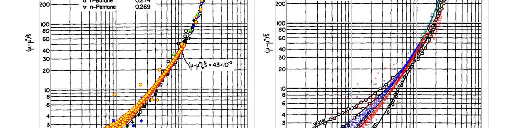
To test these assertions a small dataset was compiled and plotted against the results published in the original Jossi et al (1962) paper. In the Jossi et al paper, plots of reduced density against the reduced residual viscosity are shown for normal fluids (with critical compressibilities between 0.269 and 0.294) and for other fluid trends including hydrogen, water and ammonia. Measured viscosity data taken from the literature has been overlaid onto these original charts in Figure 2 so as to effect a basic validation. To achieve this the measured viscosity has been used, the Stiel-Thodos method is used for the dilute gas viscosity and the enhanced Peng-Robinson cubic equation of state is used for the density prediction. Note that this isn’t definitive as measured data is not used for all variables, but it should be sufficient to test whether the trends are reasonable.
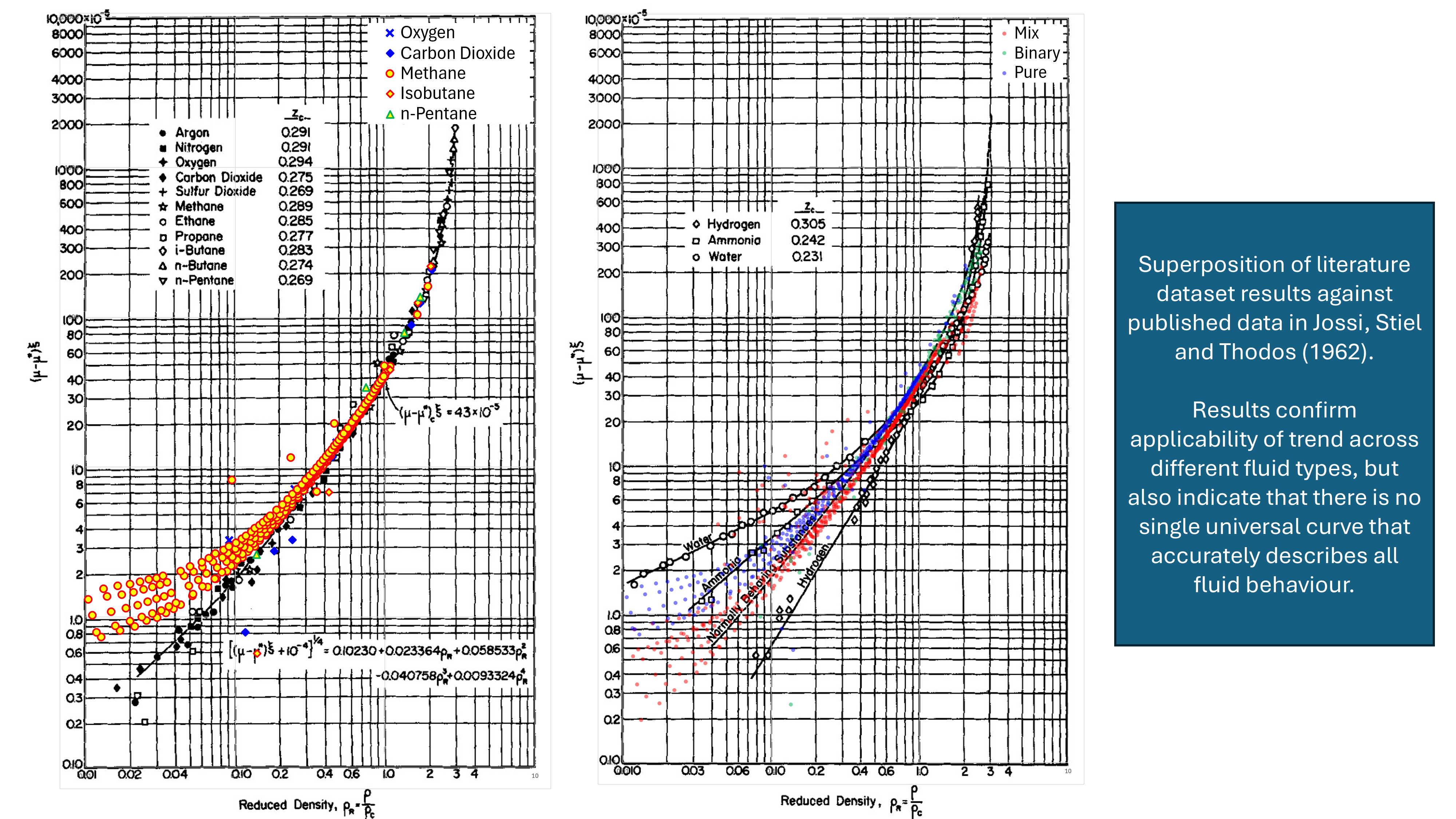
It can be seen that whilst the general trend is consistent, there is variability in the measured results. For a given reduced density, the scatter in the points plotted (across pure fluids, binary mixtures and hydrocarbon mixtures) is over an order of magnitude difference. This supports a view that for an accurate predictive result, it would be necessary to tune the regression coefficients. An advantage of the Jossi et al approach is that once tuned to a particular fluid, the equation should be suitable for extrapolation to higher and lower densities. In effect, this allows a viscosity model to be assembled from measured data that permits extrapolation and not just interpolation.
Given that the Jossi et al method used to determine the liquid mixture viscosity appears to have been derived from gas viscosity data, and was validated in Figure 2 using gas viscosity measurements, the Lohrenz, Bray and Clark suggestion that the method could be extended to gas viscosity prediction is reasonable. With current cubic equation of state techniques (including volume translation), it is now possible to obtain density for liquid and gas mixtures with equal ease. This means that the Jossi et al approach can be applied to both gases and liquids, and the Comings et al chart method is no longer required. On the other hand, given the wide scatter of points at lower reduced excess viscosity and reduced density, this may not be as robust as other techniques. Just because a method can be applied, does not necessarily mean that it should be used.
Non-monotonic Stiel-Thodos for Heavier Components
Another shortcoming of the LBC method is that, as noted by Whitson, it does not predict monotonically increasing viscosity for higher carbon numbers. Given that the LBC model is in almost ubiquitous use throughout the oil and gas industry, this was a somewhat startling revelation. I mean, really? The expected behaviour is that as the hydrocarbons get bigger in size, the viscosity should increase. A validation of the assertion can be seen in Figure 3 where liquid viscosity predictions using Pyrus’ implementation of LBC have been plotted on top of Whitson’s results. This confirms that there is a non-monotonic trend. Whitson notes that this defective behaviour can be overcome through use of a different method to estimate the component viscosities instead of Stiel-Thodos, such as group contribution methods like Orrick-Erbar.
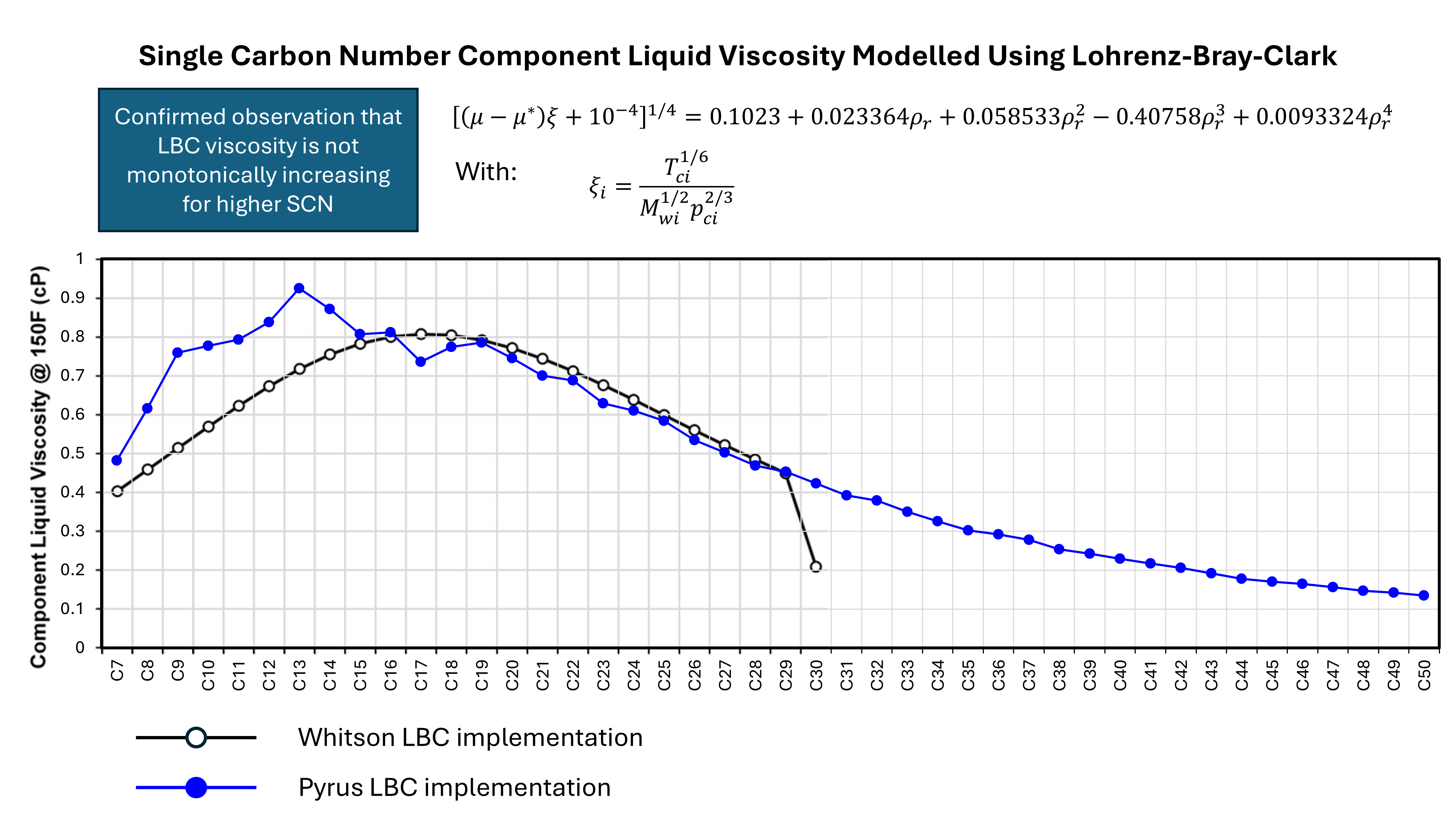
Clearly the use of LBC for hydrocarbon mixtures with any heptanes-plus components must carefully calculate the low-pressure viscosities for those components and check that their behaviour is consistent with expectations.
Density Sensitivity
Another challenge with the LBC method is that it has been noted that the predicted viscosity is sensitive to the density calculation. Accurate density predictions from the equation of state being used are essential for this method to be applied. By coupling the method to an equation of state, the method should help to produce thermodynamically consistent viscosities.
Binary Mixtures
Binary mixtures can exhibit unexpected behaviours. In moving from 100% mole fraction of one component in a binary mixture to the other, the viscosity does not always follow a monotonic trend. That is to say, the viscosity can increase and then decrease, and vice versa. The LBC method can struggle with these types of binary mixture.
Various recommended viscosity methods are described in Poling et al (2004). These include the theoretical approach of Chung and the corresponding states principle approaches of Lucas and the TRAPP (“TRAnsport Properties Prediction”) method.
A comparison of these recommended viscosity methods against the LBC approach and the ubiquitous Lee, Gonzalez and Eakin correlation approach is shown in Figure 4. This shows the experimental results for measured viscosity for the hydrogen-ammonia binary fluid (experimental data taken from Poling et al). It might be expected that this will be difficult for LBC to model accurately since the Jossi et al plot of reduced residual viscosity against reduced density shows different trends for pure ammonia and pure hydrogen (see right-hand chart in Figure 2 that clearly shows the separation between ammonia and hydrogen according to the data from Jossi et al).
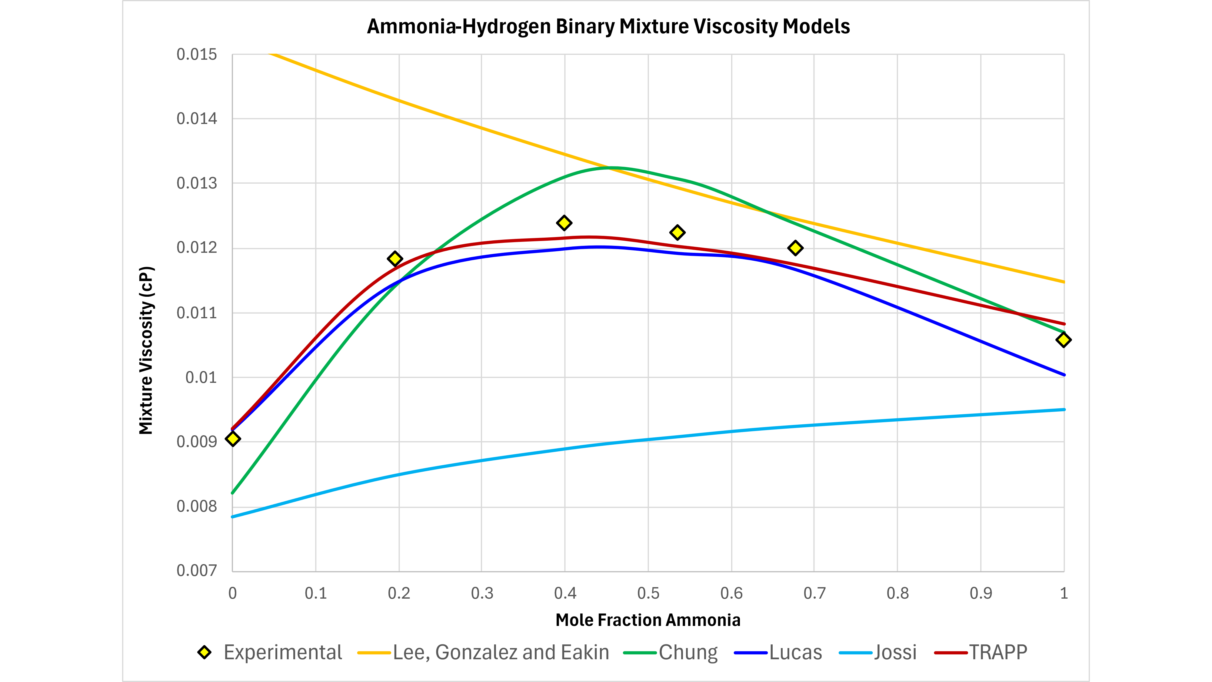
It can be seen that all of the recommended approaches capture the non-monotonic behaviour and that both the Lee, Gonzalez and Eakin, and the Lohrenz, Bray and Clark approaches both fail to capture the correct behaviour. This suggests that whilst a tuned LBC approach may be appropriate where experimental data are available to build a suitable viscosity model, in general other viscosity approaches may be more suitable for predictive viscosity modelling. This is particularly important to consider when no experimental data are available.
References
- Comings, E. W., Mayland, B. J., and Egly, R. S. 1944. The Viscosity of Gases at High Pressures. University of Illinois Engineering Experiment Station Bulletin No. 354.
- Herning, F. and Zipperer, L. 1936. Beitrag zur Berechnung der Zähigkeit Technischer Gasgemische aus den Zähigkeitswerten der Einzelbestandteile (Calculation of the Viscosity of Technical Gas Mixtures from Viscosity of the individual Gases), Gas und Wasserfach 79: 49–54, 69-73.
- Jossi, J. A., Stiel, L. I., and Thodos, G. 1962. The Viscosity of Pure Substances in the Dense Gaseous and Liquid Phases. AIChE Journal 8: 59-63. https://doi.org/10.1002/aic.690080116.
- Lee, A. L., Gonzalez, M. H., and Eakin, B. E. 1966. The Viscosity of Natural Gas. J Pet Technol 18 (8): 997-1000. SPE-1340-PA. https://doi.org/10.2118/1340-PA.
- Lohrenz, J., Bray, B.G., and Clark, C.R. 1964. Calculating Viscosities of Reservoir Fluids From Their Compositions. J Pet Technol 16 (10): 1171–1176. SPE-915-PA. https://doi.org/10.2118/915-PA.
- Poling, B. E., Prausnitz, J. M., and O’Connell, J. P. 2004. The Properties of Gases and Liquids, fifth edition. New York: McGraw-Hill Book Co.