The Lucas corresponding states method for viscosity has been around for nearly fifty years. As shown in this blog post, the predictive performance of the method is impressive and it is relatively straightforward to implement. As such it appears to be a solid and reliable choice to use for prediction of gas viscosities.
Many gas viscosity prediction methods depend on corresponding States. Corresponding states is a recognised principle that should be familiar to most petroleum engineers as it forms the foundation of the classical Z-factor correlation chart first published by Standing and Katz (1942). The general principle is that all gases comprise randomly moving molecules which interact with each other through collisions. Once the molecular size and attraction / repulsion are adjusted for, all components should in theory behave similarly in relation to their critical point. Thus by expressing temperature and pressure in terms of reduced temperature (T/Tc) and reduced pressure (p/pc), any component with the same reduced temperature and reduced pressure (a corresponding state) should have the same Z-factor.
Similarly, for a corresponding state of reduced temperature and reduced pressure, any component should have the same reduced viscosity (μ/μc). If we can accurately model the viscosity for a reference component, then we can easily determine the viscosity for any other component, provided the critical point properties for the component are known.
Corresponding States Principle
A direct application of the principle of corresponding states is that defined by Pedersen et al.. This compares a component’s critical pressure, temperature and the molecular weight to the same properties of a reference fluid. The relationships between the properties are used to first determine the equivalent temperature and pressure conditions that should be used to determine the reference fluid viscosity, and this is then further adjusted by the reduced viscosity. Pedersen also propose relationships from which the pseudo-critical properties for mixtures can be determined, thus allowing their method to be applied to both pure components and mixtures.
Originally, as implemented in Pyrus, the accuracy of the Pedersen method did not replicate the published results. This turned out to be an issue with the code itself rather than the method. The consequence was that other corresponding states methods were examined, including that of Lucas. The Lucas method is effective, and at the time it was first implemented, it lent weight to the assertion that it was the Pyrus-specific implementation of the Pedersen method that was flawed rather than the corresponding states technique itself.
Lucas Method
Outline Principles
Going back to first principles we utilise the kinetic theory of gases to model the collisions between randomly moving molecules. We can solve for viscosity by considering collisions between molecules that are assumed to be rigid non-attractive spheres to obtain the relationship:
\[\mu=\frac{26.69(MT)^{1/2}}{\sigma^2} \label{eq:rigid_sphere}\]Where:
- μ = gas viscosity (µP)
- M = molecular weight (g/mol)
- T = temperature (K)
- σ = hard-sphere diameter (Å)
The Pyrus implementation of Chapman-Enskog theory uses the method of Chung et al. In this approach the hard sphere diameter is modelled as a function of the cube-root of the critical volume. This can be expressed as:
\[\sigma^3=f(V_c) \label{eq:sigma_vc}\]Instead we can follow the approach of Lucas (1974) and define the critical volume based on ideal gas theory:
\[V_c \propto RT_c/p_c \label{eq:vc_ideal_gas}\]By combining equations \(\ref{eq:sigma_vc}\) and \(\ref{eq:vc_ideal_gas}\) with equation \(\ref{eq:rigid_sphere}\) we can express a dimensionless viscosity for low-pressure as:
\[\mu_r=\xi\mu=f(T_r) \label{eq:lucas_dimensionless_viscosity}\]With:
\[\xi=\left[\frac{(RT_c)(N_o)^2}{M^3P_c^4}\right]^{1/6} \label{eq:lucas_xi}\]Where:
- ξ = reduced, inverse viscosity (m2/N·s)
- R = gas constant = 8314.46261815324 J/(kmol·K)
- No = Avogadro’s number = 6.02214076 × 1026 (kmol)-1
- Tc = critical temperature (K)
- pc = critical pressure (N/m2)
This can also be expressed in more convenient units as:
\[\xi=0.176423\left(\frac{T_c}{M^3P_c^4}\right)^{1/6} \label{eq:lucas_inverse_viscosity}\]Where:
- ξ = reduced, inverse viscosity (µP)-1
- R = gas constant = 8.31446261815324 J/(mol·K)
- No = Avogadro’s number = 6.02214076 × 10²³ (mol)-1
- Tc = critical temperature (K)
- pc = critical pressure (bar)
In the published literature the constant in equation \(\ref{eq:lucas_inverse_viscosity}\) is usually given as 0.176. The more accurate value shown (and an even more precise value used in Pyrus) are determined through manipulation of the units in equation \(\ref{eq:lucas_xi}\) and application of the exact gas constant and Avogadro number. Whilst there is some truth to the notion that this is unnecessary precision, the fact remains that the gas constant and Avogadro’s number are defined decimal quantities. When programming the constant in Java as a double precision constant, the same memory is consumed whether the constant is stated to three decimal places, or to the limits of double precision accuracy. Therefore there is no compelling reason not to program and use the exact constant as follows:
/**
 * Constant in Lucas reduced, inverse viscosity equation.
 */
private static final double LUCAS_CONST = (pow((Mixture.GAS_CONSTANT_SI * 1000.0
        * pow(PseudoComponent.AVOGADRO_NUMBER, 2.0)) / (pow(100000.0, 4.0)), 1.0 / 6.0)) / 1000000.0
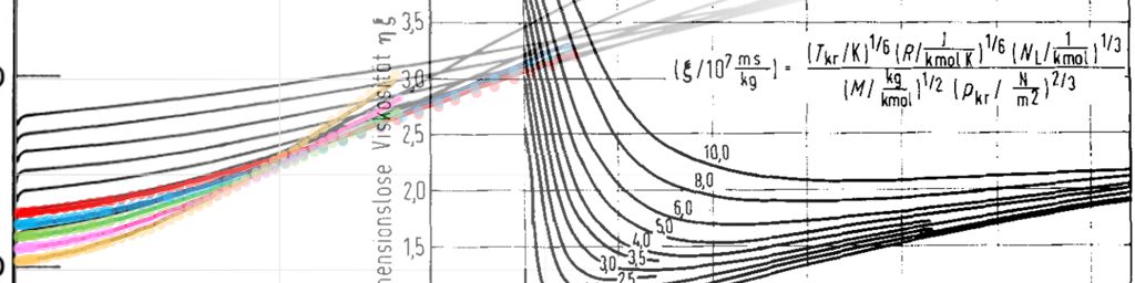
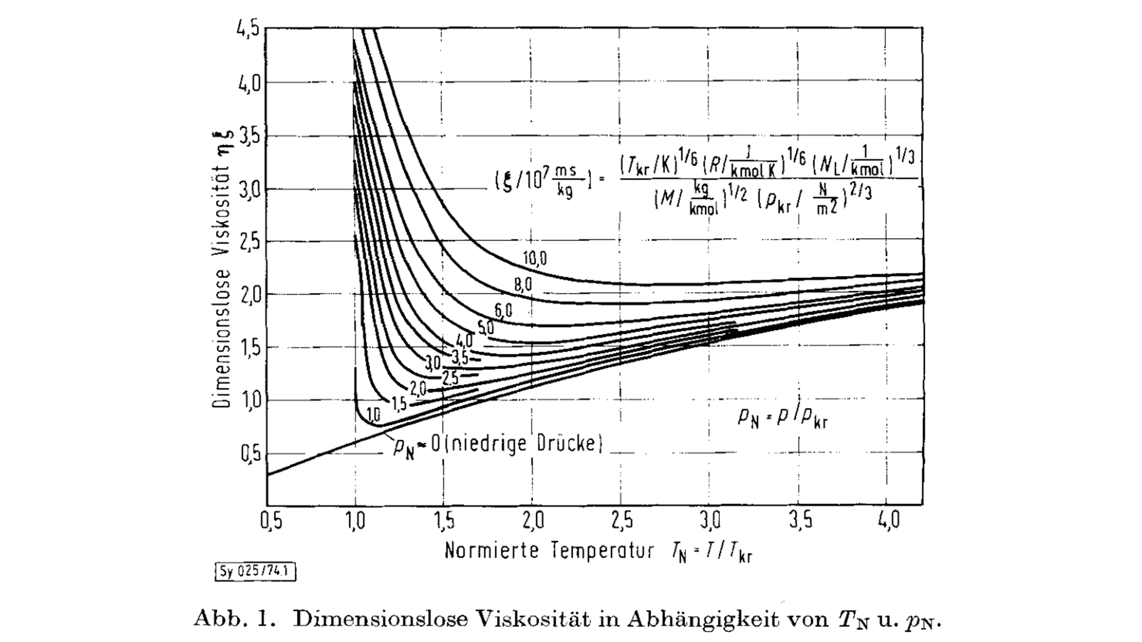
This leads to a relationship between dimensionless viscosity as a function of the reduced temperature and pressure as shown in Figure 1 (figure taken from the Lucas, 1974 paper).
Detailed Workflow
Original published papers for the Lucas method are surprisingly hard to come by. Instead, for application of this principle to gas mixtures at low and high pressures, the approaches outlined in Poling et al (2004) and Kleiber and Joh (2010) are used. The first step is to define the reduced viscosity as the product of the low-pressure viscosity and inverse viscosity in terms of Tr in a manner consistent with equation \(\ref{eq:lucas_dimensionless_viscosity}\).
\[Z_1=\mu^o\xi=\left[0.807T_r^{0.618}-0.357e^{(-0.449T_r)}+0.340e^{(-4.058T_r)}+0.018\right]F_P^oF_Q^o\]Where:
- ξ = reduced, inverse viscosity (µP)-1 as per equation \(\ref{eq:lucas_xi}\)
- μo = low-pressure viscosity (µP)
- Tr = reduced temperature = T / Tc (dimensionless)
With:
\[\begin{eqnarray} F_P^o = \begin{cases} 1 & ( 0\le\mu_r\lt0.022 ) \\ 1+30.55(0.292-Z_c)^{1.72} & ( 0.022\le\mu_r\lt0.075 ) \\ 1+30.55(0.292-Z_c)^{1.72}|0.96+0.1(T_r-0.7)| & ( 0.075\le\mu_r ) \end{cases} \end{eqnarray}\] \[F_Q^o=1.22Q^{0.15}\left\{1+0.00385\left[(T_r-12)^2\right]^{1/M}sign(T_r-12)\right\}\] \[\mu_r=52.46\frac{\mu^2p_c}{T_c^2} \label{eq:lucas_reduced_dipole}\]Where:
- FPo = polarity correction factor
- FQo = quantum correction factor (only for quantum gases He = 1.38, H2 = 0.76 and D2 = 0.52)
- μr = reduced dipole moment (dimensionless) different to the reduced dipole method of Chung
The function sign() indicates that a value of +1 or −1 should be used depending on whether the variable passed to the function is positive or negative.
To establish gas viscosity at high-pressure we next calculate Z2:
\[\begin{eqnarray} Z_2 = \begin{cases} 0.6 + 0.76P_r^\alpha+(6.99P_r^\beta-0.6)(1-T_r) & ( T_r\le1.0 , P_r \lt (p_{vp}/p_c) ) \\ Z_1Y^* & ( 1 \lt T_r \lt 40, 0 \lt p_r \lt 100 ) \end{cases} \end{eqnarray}\]With:
\[\alpha=3.262+14.98p_r^{5.508}\] \[\beta=1.39+5.746P_r\] \[Y^*=\left[1+\frac{ap_r^e}{bp_r^f+\left(1+cP_r^d\right)^{-1}}\right]\] \[a=\frac{a_1}{T_r}e^{a_2T_r^\gamma}\] \[b=a(b_1T_r-b_2)\] \[c=\frac{c_1}{T_r}e^{c_2T_r^\delta}\] \[d=\frac{d_1}{T_r}e^{d_2T_r^\varepsilon}\] \[e=e_1\] \[f=f_1e^{f_2T_r^\zeta}\]The constants in the pressure correction term is similar to that proposed by Reichenberg. Although Reichenberg’s method is not covered in the blog post, a comparison of the terms is shown in the table below. The similarity between many of the constants suggests that the differences arise mainly as a result of the different datasets used to establish the constants.
| Constant | Lucas | Reichenberg |
|---|---|---|
| \(a_1\) | 1.245 × 10⁻³ | 1.9824 × 10⁻³ |
| \(a_2\) | 5.1726 | 5.2683 |
| \(\gamma\) | −0.3286 | −0.5767 |
| \(b_1\) | 1.6553 | 1.6552 |
| \(b_2\) | 1.2723 | 1.276 |
| \(c_1\) | 0.4489 | 0.1319 |
| \(c_2\) | 3.0578 | 3.7035 |
| \(\delta\) | −37.7332 | −79.8678 |
| \(d_1\) | 1.7368 | 2.9496 |
| \(d_2\) | 2.231 | 2.919 |
| \(\varepsilon\) | −7.6351 | −16.6169 |
| \(e_1\) | 1.3088 | 1.5 |
| \(f_1\) | 0.9425 | 1 |
| \(f_2\) | −0.1853 | 0 |
| \(\zeta\) | 0.4489 | 0 |
Polar and quantum correction factors are applied as:
\[\mu=\frac{Z_2F_PF_Q}{\xi}\]With:
\[F_P=\frac{1+(F_P^o-1)Y^{-3}}{F_P^o}\] \[F_Q=\frac{1+\left(F_Q^o-1\right)\left[Y^{-1}-0.007(\ln Y)^4\right]}{F_Q^o}\] \[\begin{eqnarray} Y = \begin{cases} Z_2/Z_1 & ( T_r\le1.0 , P_r \lt (p_{vp}/p_c) ) \\ Y^* & ( 1 \lt T_r \lt 40, 0 \lt p_r \lt 100 ) \end{cases} \end{eqnarray}\]Mixing rules for the Lucas approach are straightforward and generally follow Kay’s mixing rules:
\[T_{cm}=\sum_{i=1}^ny_iT_{ci}\] \[p_{cm}=RT_{cm}\frac{\sum_{i=1}^ny_iZ_{ci}}{\sum_{i=1}^ny_iV_{ci}}\] \[M_{m}=\sum_{i=1}^ny_iM_{i}\] \[F_{Pm}^o=\sum_{i=1}^ny_iF_{Pi}^o\] \[F_{Qm}^o=\left(\sum_{i=1}^ny_iF_{Qi}^o\right)A\]With:
\[\begin{eqnarray} A = \begin{cases} 1-0.01\left(\frac{M_H}{M_L}\right)^{0.87} & ( \frac{M_H}{M_L} \gt 9, 0.05\lt\gamma_H\lt0.7 ) \\ 1 & ( otherwise ) \end{cases} \end{eqnarray}\]Where:
- H = mixture component of highest molecular weight
- L = mixture component of lowest molecular weight
Implementation in Java
The Pyrus implementation of the Lucas method is shown below. Note that Pyrus uses javax.measure units and measurements with custom oilfield units. The use of these methods should be self-explanatory for anyone trying to follow the code. The code also has a number of methods to obtain component parameters such as critical properties etc. These methods are not shown and it can be assumed that the values provided are consistent with standard data reference tables.
/**
 * Applies the corresponding states principle to determine viscosity following the method of Lucas.
 *
 * @param p mixture pressure
 * @param t mixture temperature
 * @return viscosity of the mixture
 */
public Amount<DynamicViscosity> getViscosityLucas(Amount<Pressure> p, Amount<Temperature> t) {
    double t_k = t.doubleValue(KELVIN);
    double p_bar = p.doubleValue(BAR);

    // Mixture rules
    double tc_mix_k = 0.0;
    double m_mix = 0.0;
    double yizci = 0.0, yivci = 0.0;
    for (FluidComponent fc_i : eos_composition.keySet()) {
        final Double yi = eos_composition.get(fc_i);
        tc_mix_k += yi * Amount.valueOf(fc_i.t_crit(), RANKINE).doubleValue(KELVIN);
        m_mix += yi * fc_i.mass();
        yizci += yi * fc_i.z_crit();
        yivci += yi * Amount.valueOf(fc_i.v_crit() / Mixture.MOLE_PER_LBMMOL, CUBIC_FOOT)
                .doubleValue(CUBIC_CENTIMETRE);
    }
    double pc_mix_bar = GAS_CONSTANT_SI * 10.0 * tc_mix_k * (yizci / yivci);

    // Mixture polarity and quantum correction factors
    double fop_mix = 0.0;
    double foq_mix = 0.0;
    for (FluidComponent fc_i : eos_composition.keySet()) {
        Condition crit_pt_i = fc_i.criticalPoint();
        double tc_i_k = crit_pt_i.getTemperature().doubleValue(KELVIN);
        double pc_i_bar = crit_pt_i.getPressure().doubleValue(BAR);
        double tr_i = t_k / tc_i_k;
        double zc_i = fc_i.z_crit();
        double m_i = fc_i.mass();
        double mu_i = ((PseudoComponent) fc_i).dipole();
        final double mu_r = 52.46 * (mu_i * mu_i * pc_i_bar) / (tc_i_k * tc_i_k);
        double fop_i; // correction factor for polarity effects
        if (mu_r < 0.022) {
            fop_i = 1.0;
        } else if (mu_r > 0.075) {
            fop_i = 1.0 + 30.55 * pow(0.292 - zc_i, 1.72);
        } else {
            fop_i = 1.0 + 30.55 * pow(0.292 - zc_i, 1.72) * abs(0.96 + 0.1 * (tr_i - 0.7));
        }
        double foq_i = 1.0; // correction factor for quantum effects
        final double q = ((PseudoComponent) fc_i).quantumLucas();
        if (q > 0.0) {
            final double trminustwelve = tr_i - 12;
            double sign = trminustwelve > 0.0 ? 1.0 : -1.0;
            foq_i = 1.22 * pow(q, 0.15) * (1.0 + 0.00385 * pow(pow(trminustwelve, 2.0), 1.0 / m_i) * sign);
        }
        final Double yi = eos_composition.get(fc_i);
        fop_mix += yi * fop_i;
        foq_mix += yi * foq_i;
    }
    double mh = getHeaviestComponent(eos_composition).mass();
    double ml = getLightestComponent(eos_composition).mass();
    double a = 1.0;
    if ((mh / ml) > 9.0) {
        double gammah = getHeaviestComponent(eos_composition).specificGravityWater();
        if (gammah > 0.05 && gammah < 0.7) {
            a = 1.0 - 0.01 * pow(mh / ml, 0.87);
        }
    }
    foq_mix *= a;

    // Calculate dense gas mixture viscosity.
    final double tr = t_k / tc_mix_k; // reduced temperature
    final double pr = p_bar / pc_mix_bar; // reduced pressure
    double mpow3 = pow(m_mix, 3.0);
    double pcpow4 = pow(pc_mix_bar, 4.0);
    double xi = 0.176 * pow(tc_mix_k / (mpow3 * pcpow4), 1.0 / 6.0); // reduced, inverse viscosity

    // First calculate a parameter Z_1
    double z_one = (0.807 * pow(tr, 0.618) - 0.357 * exp(-0.449 * tr) + 0.340 * exp(-4.058 * tr) + 0.018)
            * fop_mix * foq_mix;

    // Next calculate Z_2
    Condition crit_pt = new Condition(Amount.valueOf(tc_mix_k, KELVIN), Amount.valueOf(pc_mix_bar, BAR));
    double z_two = PseudoComponent.gasViscosityHighPressure(z_one, p, t, crit_pt);

    // After computing Z_1 and Z_2 we define Y and the correction factors F_P and F_Q.
    double y = z_two / z_one;
    double fp = (1.0 + (fop_mix - 1.0) * pow(y, -3.0)) / (fop_mix);
    double fq = (1.0 + (foq_mix - 1.0) * ((1.0 / y) - 0.007 * pow(log(y), 4.0))) / (foq_mix);
    double eta_micropoise = (z_two * fp * fq) / xi; // viscosity in microPoise
    Amount<DynamicViscosity> mu_cp = Amount.valueOf(eta_micropoise / 10000.0, CENTIPOISE);
    return mu_cp;
}
The method above applies the mixing rules and then calls the static PseudoComponent.gasViscosityHighPressure method. This PseudoComponent.gasViscosityHighPressure method is implemented as follows:
/**
 * High pressure gas viscosity for this component. For reduced temperatures less than 1.0, the Lucas corresponding
 * states method is applied.
 *
 * @param z_one dilute gas viscosity in centiPoise
 * @param p pressure
 * @param t temperature
 * @param crit_pt critical point for this component or pseudo-component
 * @return viscosity of the component in centiPoise
 */
public static double gasViscosityHighPressure(double z_one, Amount<Pressure> p, Amount<Temperature> t,
        Condition crit_pt) {
    final double p_psia = p.doubleValue(POUND_PER_SQUARE_INCH);
    final double t_degr = t.doubleValue(RANKINE);
    double p_c = crit_pt.getPressure().doubleValue(POUND_PER_SQUARE_INCH);
    double t_c = crit_pt.getTemperature().doubleValue(RANKINE);
    double p_r = p_psia / p_c;
    double t_r = t_degr / t_c;

    // Calculate the dilute gas viscosity and adjust to higher pressure using method of Lucas.
    double mu_adj_highp = 0.0;
    if (t_r < 1.0) {
        PureComponent ref_fluid = PureComponent.C3H8;
        final double pc_ref_bar = Amount.valueOf(ref_fluid.p_crit(), POUND_PER_SQUARE_INCH).doubleValue(BAR);
        final double tc_ref_k = Amount.valueOf(ref_fluid.t_crit(), RANKINE).doubleValue(KELVIN);
        double tdash_ref_k = t_r * tc_ref_k;
        double pvap_ref_bar = Amount.valueOf(ref_fluid.vapourPressure(Amount.valueOf(tdash_ref_k, KELVIN)
                .doubleValue(RANKINE)), POUND_PER_SQUARE_INCH).doubleValue(BAR);
        double pr_threshold = pvap_ref_bar / pc_ref_bar;
        if (p_r < pr_threshold) {
            double alpha = 3.262 + 14.98 * pow(p_r, 5.508);
            double beta = 1.39 + 5.746 * p_r;
            mu_adj_highp = 0.6 + 0.76 * pow(p_r, alpha) + (6.99 * pow(p_r, beta) - 0.6) * (1.0 - t_r);
        } else {
            mu_adj_highp = PVT.gasViscosityHighPressureLucas(z_one, p_r, t_r);
        }
    } else if (t_r < 40.0 && p_r <= 100.0) {
        mu_adj_highp = PVT.gasViscosityHighPressureLucas(z_one, p_r, t_r);
    }
    return mu_adj_highp;
}
The method above in turn calls the static PVT.gasViscosityHighPressureLucas method. This PVT.gasViscosityHighPressureLucas method follows the approach of Lucas and is implemented as follows:
/**
 * Gas viscosity correlation to convert from low pressure viscosity to account for effect of pressure and
 * temperature. Valid in the range 1 < tr < 40 and 0 < pr <= 100.
 *
 * @param mu_atm low pressure viscosity in centiPoise
 * @param p_pr pseudo-reduced pressure
 * @param t_pr pseudo-reduced temperature
 * @return adjusted gas dynamic viscosity in centiPoise
 */
public static double gasViscosityHighPressureLucas(double mu_atm, double p_pr, double t_pr) {
    double a = (1.245e-03 * exp(5.1726 * pow(t_pr, -0.3286))) / t_pr;
    double b = a * (1.6553 * t_pr - 1.2723);
    double c = (0.4489 * exp(3.0578 * pow(t_pr, -37.7332))) / t_pr;
    double d = (1.7368 * exp(2.2310 * pow(t_pr, -7.6351))) / t_pr;
    double e = 1.3088;
    double f = 0.9425 * exp(-0.1853 * pow(t_pr, 0.4489));
    double ratio = 1.0 + (a * pow(p_pr, e)) / (b * pow(p_pr, f) + 1.0 / (1.0 + c * pow(p_pr, d)));
    return mu_atm * ratio;
}
Predictive Quality
In order to test the quality of the implemented code and check the performance of the Lucas method, the predicted viscosities of various fluids have been calculated and compared against measured data. These are the same datasets used for testing the predictive performance with the Chung et al method, and will be used for other comparisons in the future, thus providing for a consistent basis of comparison.
Pure Fluids
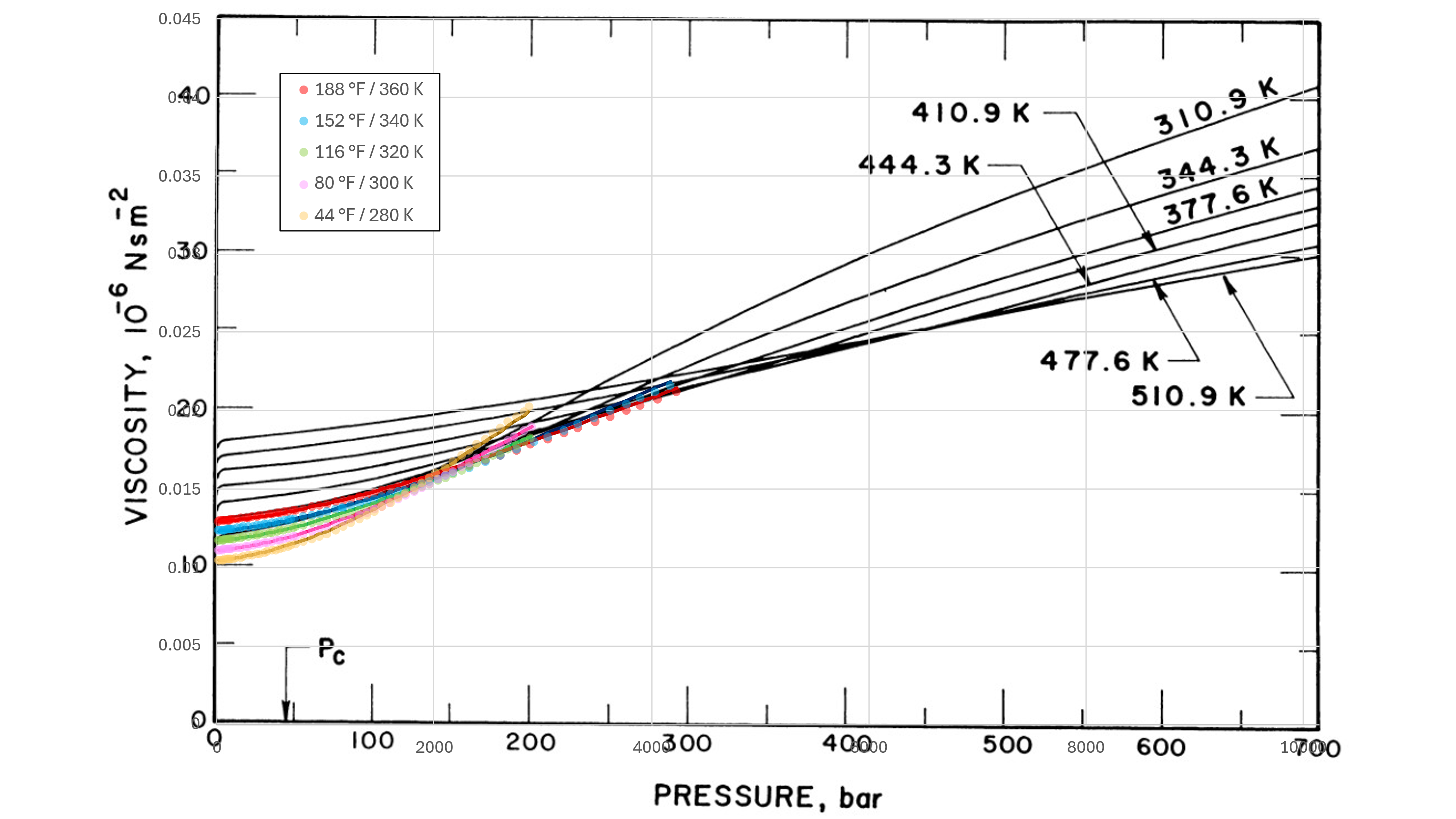
Data for methane at different temperature and pressure published by Schley et al (2004) has been compared against the implemented Lucas method. The results have also been superimposed on chart of methane viscosity data from Stephan and Lucas (1979). This is shown in Figure 2 below.
It can be seen that the predictive quality is good within the pressure range modelled, and for pure fluids in particular the Lucas method appears to be one of the best gas viscosity approaches. Further modelling should be undertaken to examine the range of performance for the Lucas method with pure fluids across a wider range of fluids.
Binary Mixtures
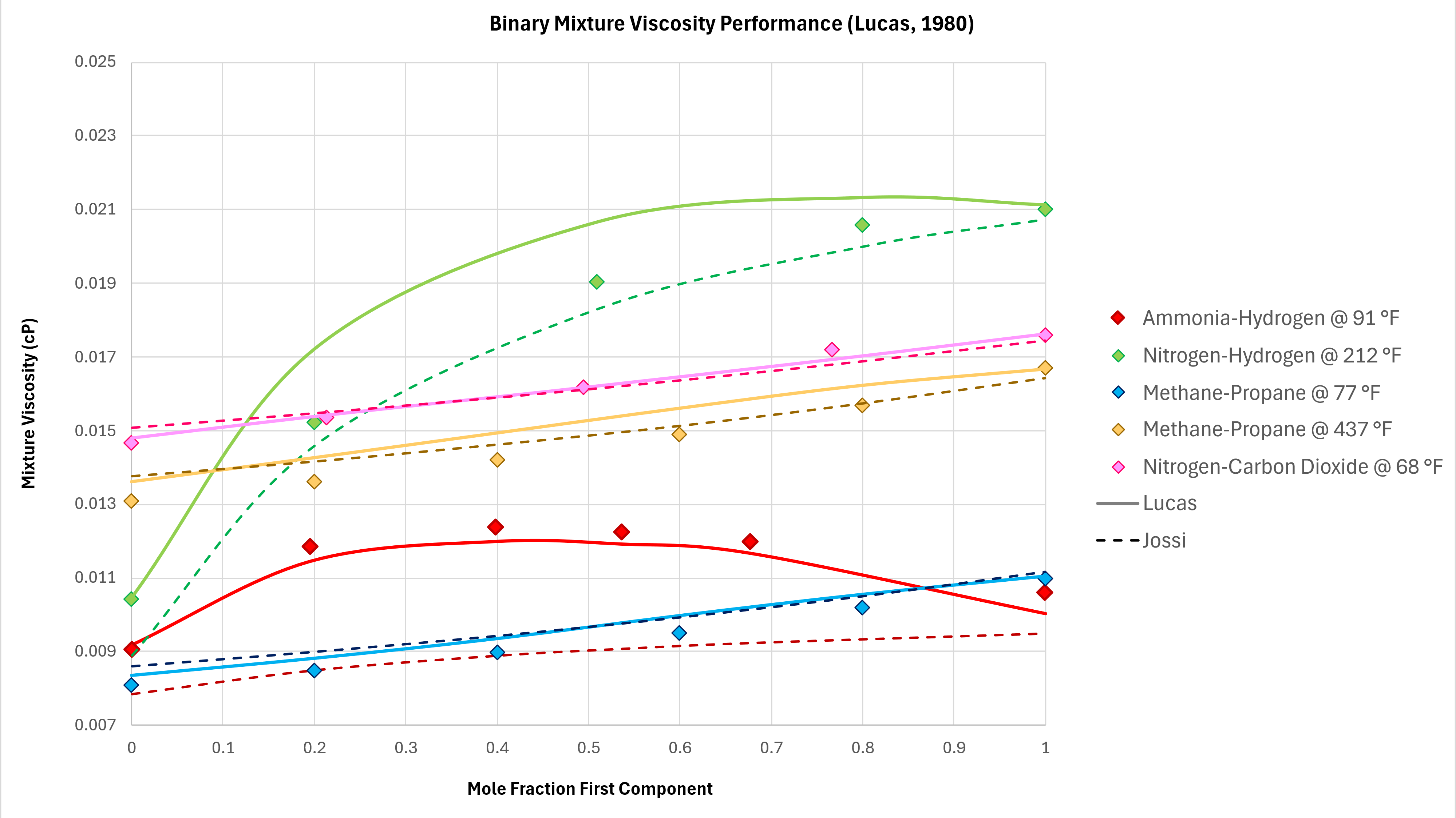
Binary mixtures can exhibit unexpected behaviours. In moving from 100% mole fraction of one component in a binary mixture to the other, the viscosity does not always follow a monotonic trend. That is to say, the viscosity can increase and then decrease, and vice versa. Various binary mixture measured viscosity data is compared against the implemented Lucas method using data taken from Poling et al (2004) as shown in Figure 3 below. All data is measured at atmospheric pressure.
The Lucas method is able to capture the non-monotonic behaviour of the Ammonia-Hydrogen binary mixture, and has good predictive capability for Methane-Propane at different temperatures. However, it is noted that the prediction of the methane-propane binary mixtures is inferior to that of the Chung et al method.
As a comparison the Jossi, Stiel and Thodos (JST) method (as used in Lohrenz-Bray-Clark) is also shown on these charts. The JST method is generally similar in performance to the Lucas method, with the exception of the Ammonia-Hydrogen binary where JST does not capture the change in viscosity vs composition accurately.
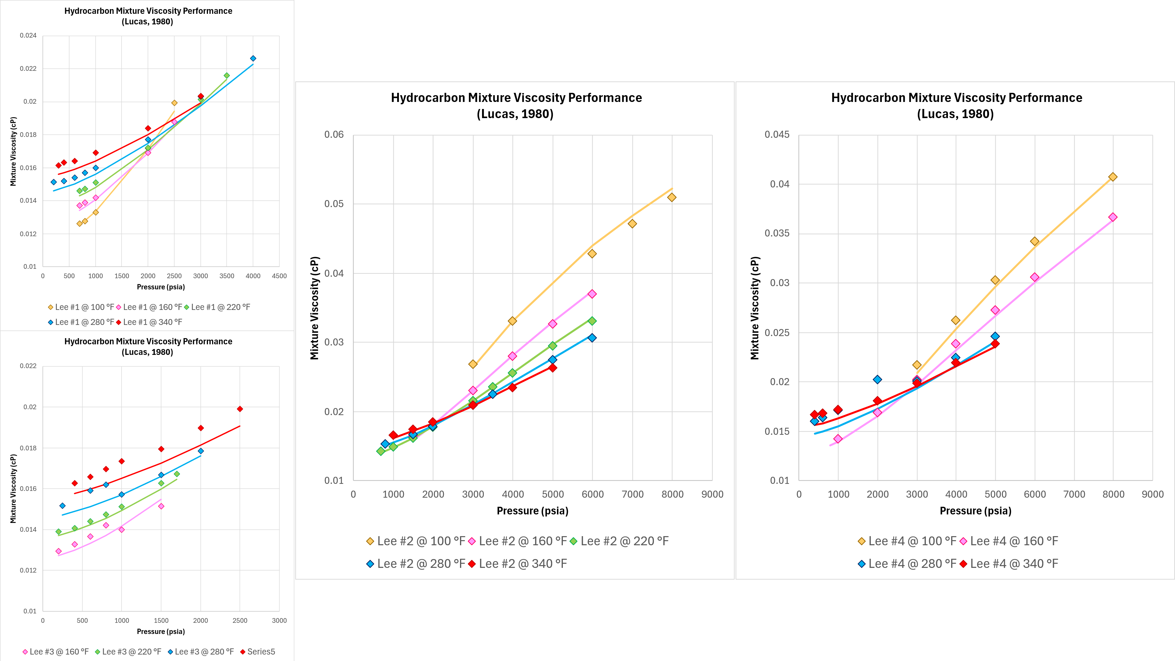
Hydrocarbon mixtures
Good performance with pure components and binary mixtures means nothing if the technique does not work on real-world fluids. Four different hydrocarbon gas mixtures and measurements of viscosity were published by Lee, Gonzalez and Eakin (1966). Whilst there are some apparent discontinuities in the measured data, this dataset is sufficient to assess the predictive performance of the implemented Lucas method as shown in Figure 5 below.
It can be seen that the Lucas method is able to model the correct trends in terms of the viscosity variation with temperature and pressure, and the absolute viscosity predicted is close to the measured values. The accuracy in all cases is superior to that observed with the Chung et al method.
References
- Chung, T. H., Ajlan, M., Lee, L. L., and Starling, K. E. 1988. Generalized Multiparameter Correlation for Nonpolar and Polar Fluid Transport Properties. Ind Eng Chem Res 27: 671-679. https://doi.org/10.1021/ie00076a024.
- Kleiber, M. and Joh, R. 2010. Calculation Methods for Thermophysical Properties. In VDI Heat Atlas, second edition, ed. VDI-Gesellschaft Verfahrenstechnik und Chemieeingenieurwesen, Chap. D1, 144-145. Heidelberg: Springer. https://doi.org/10.1007/978-3-540-77877-6.
- Lee, A. L., Gonzalez, M. H., and Eakin, B. E. 1966. The Viscosity of Natural Gas. J Pet Technol 18 (8): 997-1000. SPE-1340-PA. https://doi.org/10.2118/1340-PA.
- Lucas, K. 1974. Ein einfaches Verfahren zur Berechnung der Viskositat von Gasen und Gasgemischen (A Simple Method for Calculating the Viscosity of Gases and Gas Mixtures). Chem Ing Tech 46 (4): 157. https://doi.org/10.1002/cite.330460413.
- Lucas, K. 1980. Phase Equilibria and Fluid Properties in the Chemical Industry. Proc., Second International Conference, Berlin (West), 17-21 March, 573. Frankfurt: DECHEMA.
- Pedersen, K. S. and Fredenslund, A. 1987. An Improved Corresponding States Model for the Prediction of Oil and Gas Viscosities and Thermal Conductivities. Chem. Eng. Sci. 42 (1): 182–186. https://doi.org/10.1016/0009-2509(87)80225-7.
- Poling, B. E., Prausnitz, J. M., and O’Connell, J. P. 2004. The Properties of Gases and Liquids, fifth edition. New York: McGraw-Hill Book Co.
- Schley, P., Jaeschke, M., Küchenmeister, C., and Vogel E. 2004. Viscosity Measurements and Predictions for Natural Gas. International Journal of Thermophysics 25 (6): 1623–1652. https://doi.org/10.1007/s10765-004-7726-5.
- Stephan, K. and Lucas, K. 1979. Viscosity of Dense Fluids. New York: Springer. https://doi.org/10.1007/978-1-4757-6931-9.