The TRAPP method is a sophisticated corresponding states method that was implemented in the U.S. National Institute of Standards and Technology (NIST) standard reference database 4. Whilst this NIST database has since been largely superceded by the Reference Fluid Thermodynamic and Transport Properties Database (REFPROP), the TRAPP method remains valid and relevant.
The TRAPP method does not appear to be used extensively in the oil and gas industry, with Lohrenz-Bray-Clark usually favoured if viscosity needs to be calculated within a simulator due to its relative simplicity which facilitates faster computational speed, or the Lee, Gonzalez and Eakin correlation used by laboratories. For arbitrary hydrocarbon mixtures, particularly where the C7+ fraction has been characterised into paraffins, naphthenes and aromatic components, the TRAPP method represents a robust technique for predicting the viscosity from first principles. This has many advantages in comparison to use an empirical correlation. For generation of black-oil tables which will then be used as lookup tables within a simulator, the TRAPP method is perhaps one of the most accurate methods available for prediction of gas viscosity with hydrocarbon mixtures.
Advantages of Corresponding States
Other viscosity methods discussed on this blog have used the corresponding states principle. Amongst them are the approach of Pedersen et al. and the approach of Lucas. The beauty of the corresponding states principle is that it is so much more than a mere correlation. The oil and gas industry loves empirical correlations. And a good correlation, when fit to the dataset used to build it, can provide a remarkably accurate estimate of whatever variable is being correlated against. But caution must be exercised. Rarely is a correlation mathematically well behaved outside the constraints of the range of input variables used to create the regression (or these days to train the neural net, or similar machine learning algorithm). Not so with corresponding states, because this is founded on the first principles of physics. This is the how and why the system works. It is not merely an empirical fit to observed data. It is a theory that has been tested and proven to work in practice.
The opening introduction by Huber and Hanley (1996) in their update to the TRAPP method puts it eloquently.
Here, however, the strong point of corresponding-states principles is stressed: that methods based on the principle are theoretically based and predictive, rather than empirical and correlative. Thus, while CS cannot always reproduce a set of data within its experimental accuracy, as can an empirical correlation, it should be able to represent data to a reasonable degree but, more important, do what a correlation cannot do - estimate the properties beyond the range of existing data.
The capability for the method to predict properties for fluids for which no measurements exist is incredibly powerful. Not only does it mean that the method can potentially be applied into applications for which there is not much measured data available (high-pressure high-temperature environments for example), but it can also confidently be applied to arbitrary fluid mixtures for which no measurements may have ever been made.
TRAPP Method
The TRAPP method was originally proposed by Hanley (1976) and led to a computer program known as ‘TRAnsport Properties Prediction’ (Ely and Hanley, 1981) which was concatenated to TRAPP. Modifications to the original TRAPP procedure were outlined by Huber and Hanley (1996) and this forms the basis for the approach outlined here.
Outline Principles
For a mixture of n components with composition given by {zi}, the viscosity μ at a density ρ and temperature T is considered equivalent to the viscosity of a hypothetical pure fluid. The properties of this hypothetical pure fluid are first obtained through the use of various mixing and combining rules. The hypothetical pure fluid is then considered equivalent to a reference fluid at a corresponding state given by an equivalent reference density ρ0 and and equivalent reference temperature T0. Thus:
\[\mu_{mix}(\rho, T, \{z_i\}) \equiv \mu_x(\rho, T) \equiv \mu_{ref}(\rho_o, T_o)F_{\eta}\]Where:
- μ = viscosity (µPa·s)
- ρ = density (gmol/L)
- T = temperature (K)
- Fη = reference fluid residual viscosity adjustment factor
With:
\[T_o=T/f \label{eq:equiv_f}\] \[\rho_o=\rho h \label{eq:equiv_h}\] \[F_{\eta}=\left(\frac{M}{M_{ref}}f\right)^{1/2}h^{-2/3}\]The parameters f and h are equivalent substance reducing parameters.
For a mixture the residual viscosity of the hypothetical pure fluid is obtained from the residual viscosity of the reference fluid, propane, using:
\[\mu_{mix}-\mu_{mix}^o=F_{\eta,mix}\left[\mu_{ref}-\mu_{ref}^o\right]\times10+\Delta\eta^{ENSKOG} \label{eq:trapp_mix_viscosity}\]Where:
- μmixo = mixture low-pressure viscosity (µP)
- μref − μrefo = propane (reference) residual viscosity (µPa·s)
- ΔηENSKOG = term to account for size differences (µP)
The low-pressure viscosity for the mixture can be calculated using various methods. For Pyrus the default approach is to use the Reichenberg method if groups have been defined and to fall back to the Lucas method otherwise. This is described in the following section ‘Low-pressure Viscosity Approach’. The propane reference fluid residual viscosity is given by the modified Benedict–Webb–Rubin equation of state given by Younglove and Ely (1987) as described in Poling et al (2004). It is noted that this prevents earlier problems encountered when using TRAPP due to use of methane as the reference fluid at very low temperatures. Note that in this equation the reference residual viscosity has different units to other viscosities which are given in microPoise, thus it is necessary to multiply the reference residual viscosity by 10 in equation \(\ref{eq:trapp_mix_viscosity}\).
\[\mu_{ref}-\mu_{ref}^o=G_1e^{\left[\rho_o^{0.1}G_2+\rho_o^{0.5}(\rho_{r,ref}-1)G_3\right]}-G_1 \label{eq:ref_residual_viscosity}\]With:
\[\rho_{r,ref}=\rho_o/\rho_{c,ref}\] \[G_1=e^{E_1+E_2/T_o}\] \[G_2=E_3+E_4/T_o^{1.5}\] \[G_3=E_5+\frac{E_6}{T_o}+\frac{E_7}{T_o^2}\] \[E_1=-14.113294896\] \[E_2=968.22940153\] \[E_3=13.686545032\] \[E_4=-12511.628378\] \[E_5=0.0168910864\] \[E_6=43.527109444\] \[E_7=7659.4543472\]To evaluate the reference residual viscosity it is necessary to determine the equivalent reference density ρ0 and and equivalent reference temperature T0. This is similar to equations \ref{eq:equiv_f} and \ref{eq:equiv_h}, but applied to the mixture:
\[T_o=T/f_{mix} \label{eq:equiv_f_mix}\] \[\rho_o=\rho h_{mix} \label{eq:equiv_h_mix}\]The following mixing rules are applied to determine fmix in equation \ref{eq:equiv_f_mix} and hmix in equation \ref{eq:equiv_h_mix}:
\[h_{mix}=\sum_{i=1}^{n}\sum_{j=1}^{n}z_iz_jh_{ij}\] \[f_{mix}=\frac{\sum_{i=1}^{n}\sum_{j=1}^{n}z_iz_jf_{ij}h_{ij}}{h_{mix}}\] \[h_{ij}=\frac{\left[h_i^{1/3}+h_j^{1/3}\right]^3}{8}\] \[f_{ij}=\left(f_if_j\right)^{1/2}\]With:
\[f_i=\frac{T_{c,i}}{T_{c,ref}}\left[1+\left(\omega_i-\omega_{ref}\right)\left(0.05202976-0.7498189\ln T_{r,i}\right)\right]\] \[h_i=\frac{\rho_{c,ref}Z_{c,ref}}{\rho_{c,i}Z_{c,i}}\left[1+\left(\omega_i-\omega_{ref}\right)\left(0.1435971-0.2821562\ln T_{r,i}\right)\right]\]The reference fluid residual viscosity adjustment factor Fη,mix in equation \(\ref{eq:trapp_mix_viscosity}\) is given by:
\[F_{\eta,mix}=\frac{M_{ref}^{-1/2}}{h_{mix}^2}\sum_{i=1}^{n}\sum_{j=1}^{n}z_iz_j\left(f_{ij}M_{ij}\right)^{1/2}h_{ij}^{4/3} \label{eq:f_eta_mix}\]With:
\[M_{ij}=\frac{2M_iM_j}{M_i+M_j}\]The final term in equation \(\ref{eq:trapp_mix_viscosity}\) is ΔηENSKOG which accounts for size differences between the molecules. It is given by:
\[\Delta\eta^{ENSKOG}=\eta_{mix}^{ENSKOG}-\eta_x^{ENSKOG} \label{eq:delta_enskog}\]With:
\[\eta_{mix}^{ENSKOG}=\sum_{i=1}^{n}\beta_iY_i+\alpha\rho^2\sum_{i=1}^{n}\sum_{j=1}^{n}z_iz_j\sigma_{ij}^6\eta_{ij}^og_{ij} \label{eq:eta_mix_enskog}\]Where:
- ρ = density (mol/L)
- σ = hard sphere diameter (Å)
- ηo = viscosity for a rigid, non-attracting sphere model (µP)
- gij = radial distribution function
With:
\[\alpha=\frac{48}{25\pi}\left[\frac{2\pi}{3}(6.023 \times 10^{-4})\right]^2\] \[\sigma_i=4.771h_i^{1/3}\] \[\sigma_{ij}=\frac{\sigma_i+\sigma_j}{2}\] \[\eta_{ij}^o=26.69\frac{\left(M_{ij}T\right)^{1/2}}{\sigma_{ij}^2}\] \[g_{ij}=\frac{1}{1-\xi}+\frac{3\xi}{(1-\xi)^2}\Theta_{ij}+\frac{2\xi^2}{(1-\xi)^3}\Theta_{ij}^2\] \[\Theta_{ij}=\frac{\sigma_i\sigma_j}{2\sigma_{ij}}\frac{\sum_{k=1}^{n}z_k\sigma_k^2}{\sum_{k=1}^{n}z_k\sigma_k^3}\] \[\xi=(6.023 \times 10^{-4})\frac{\pi}{6}\rho\sum_{i=1}^{n}z_i\sigma_i^3\] \[Y_i=z_i\left[1+\frac{8\pi}{15}(6.023 \times 10^{-4})\rho\sum_{j=1}^{n}z_j\left(\frac{M_j}{M_i+M_j}\right)\sigma_{ij}^3g_{ij}\right]\]The n values of βi are obtained by solving the n systems of linear equations given by:
\[\sum_{j=1}^{n}B_{ij}\beta{ij}=Y_i\]With:
\[B_{ij}=2\sum_{k=1}^{n}z_iz_k\frac{g_{ik}}{\eta_{ik}^o}\left(\frac{M_k}{M_i+M_k}\right)^2\left[\left(1+\frac{5M_i}{3M_k}\right)\delta_{ij}-\frac{2M_i}{3M_k}\delta_{ij}\right]\]Where:
- δij = Kronecker delta function, 1 if i = j and 0 if i ≠ j
The quantity ηxENSKOG in equation \ref{eq:delta_enskog} is the Enskog viscosity as determined by equation \ref{eq:eta_mix_enskog} for a single component pure hypothetical fluid that has the same density ρ as the mixture. For equation \ref{eq:eta_mix_enskog} the hypothetical pure fluid has the following hard sphere diameter σx and molecular weight Mx:
\[\sigma_x=\left(\sum_{i=1}^{n}\sum_{j=1}^{n}z_iz_j\sigma_{ij}^3\right)^{1/3}\] \[M_x=\left[\sum_{i=1}^{n}\sum_{j=1}^{n}z_iz_jM_{ij}^{1/2}\sigma_{ij}^4\right]^2\sigma_x^{-8}\]Using the reference residual viscosity from equation \ref{eq:ref_residual_viscosity}, the reference fluid viscosity adjustment factor from equation \ref{eq:f_eta_mix}, and the Enskog viscosity delta from equation \ref{eq:delta_enskog} it is now possible to determine the mixture residual viscosity with equation \ref{eq:trapp_mix_viscosity}. Using the mixture residual viscosity, the actual mixture viscosity is found by adding the mixture residual viscosity to the low-pressure mixture viscosity.
Determination of the low-pressure mixture viscosity is the subject of the next section.
Low-Pressure Viscosity Approach
Low-pressure mixture viscosity generally follows the following procedure:
- For each component in the mixture, determine the pure component low-pressure viscosity using a method such as that proposed by Chung (theoretical Chapman-Enskog approach), Lucas (corresponding states approach) or Reichenberg (group contribution approach).
- Combine the pure component low-pressure viscosities using a mixing rule such as Reichenberg, Wilke or Herning and Zipperer.
In Pyrus the Reichenberg methods are generally used. This approach has been chosen as it means low-pressure viscosity for the C7+ fraction can be determined using a group contribution method which should help capture the PNA characteristics of that fraction. The Reichenberg mixing rule is used as they are considered amongst the most accurate of the mixing rules, albeit at the expense of increased complexity.
Reichenberg Pure Component Low-Pressure Viscosity
Reichenberg’s approach to determine low-pressure gas viscosity is taken from Poling et al (2004). The method is a corresponding states approach that uses a group contribution method. Low-pressure viscosity is given by:
\[\mu=\frac{M^{1/2}T}{a^*\left[1+(4/T_c)\right]\left[1+0.36T_r(T_r-1)\right]^{1/6}}\frac{T_r(1+270\mu_r^4)}{T_r+270\mu_r^4} \label{eq:reichenberg_lowp_viscosity}\]Where:
- M = molecular weight (g/mol)
- T = temperature (K)
- Tc = critical temperature (K)
- μr = reduced dipole moment (dimensionless) as per method of Lucas
With:
\[a^*=\sum_{i=1}^{n}n_iC_i\]Where:
- ni = number of groups of the ith type
- Ci = group contribution as per table
There are 28 defined groups in the Reichenberg method. For the moment Pyrus primarily uses group contribution methods for the enhanced predictive Peng-Robinson equation of state, and so only these groups and their mapping to Reichenberg’s groups are shown. If the groups used in Pyrus are not available, this is shown as “N/a”. Generally, all the groups that a C7+ pseudocomponent are broken down into are represented. The exception is the )>C<( (R) group which is not included in the Reichenberg groups. In the Pyrus scheme this is usually a very small constituent fraction, and thus a group contribution of 0.00 has been assumed. This seems a reasonable assumption given that the value lies between >C< and >C< (R) group contributions.
| Group | Group Description | Ci |
|---|---|---|
| -CH3 | Methyl group comprising one carbon atom bonded to three hydrogen atoms as part of a paraffinic chain. | 9.04 |
| -CH2- | Methylene group comprising one carbon atom bonded to two hydrogen atoms plus two single bonds as part of a paraffinic chain. | 6.47 |
| >CH- | Carbon-hydrogen group comprising one carbon atom bonded to one hydrogen atom plus three single bonds as part of a paraffinic chain. | 2.67 |
| >C< | Single carbon atom group with four single bonds as part of a paraffinic chain. | −1.53 |
| CH4 | Methane group comprising one carbon atom bonded to four hydrogen atoms. | N/a |
| C2H6 | Ethane group comprising two methyl groups bonded together. | N/a |
| )>CH (Raro) | Carbon-hydrogen group comprising one carbon atom bonded to one hydrogen atom as part of an aromatic ring. | 5.90 |
| )>C- (Raro) | Single carbon atom group as part of an aromatic ring plus a single bond. | 3.59 |
| )>C<( (Rfused) | Fused carbon atom group as part of fused aromatic (polyaromatic) rings. | 0.00 |
| >CH2 (Rcyc) | Methylene group comprising one carbon atom bonded to two hydrogen atoms as part of a cyclic ring plus two single bonds. | 6.91 |
| >CH- (Rcyc) | Carbon-hydrogen group comprising one carbon atom bonded to one hydrogen atom as part of a cyclic ring plus a single bond. | 1.16 |
| >C< (Rcyc) | Single carbon atom group as part of a cyclic ring plus two single bonds. | 0.23 |
| CO2 | Carbon dioxide group comprising a single carbon atom bonded to two oxygen atoms. | N/a |
| N2 | Nitrogen group comprising two nitrogen atoms bonded together. | N/a |
| H2S | Hydrogen sulphide group comprising a single hydrogen atom bonded to two sulphur atoms. | N/a |
If a component cannot be fully broken down into recognised groups, then Pyrus will revert to the Lucas corresponding states method. This method is chosen because testing (by myself and published results) shows that the method has excellent predictive performance for pure components.
Reichenberg Low-Pressure Viscosity Mixing Rule
Mixing rules can be determined through consideration of kinetic theory of Chapman and Enskog. This is a theoretical approach, and usually a simplification of the rigorous expressions are used. Reichenberg’s method is one such approach and it is described as incorporating elements of the kinetic theory approach of Hirschfelder et al (1954) together with corresponding states principles.
The mixture viscosity is given as:
\[\mu_{mix}=\sum_{i=1}^{n}K_i\left(1+2\sum_{j=1}^{i-1}H_{ij}K_j+\sum_{j=1\ne i}^{n}\sum_{k=1\ne i}^{n}H_{ij}H_{ik}K_jK_k\right)\]With:
\[K_i=\frac{z_i\mu_i}{z_i+\mu_i\sum_{k=1\ne i}^{n}z_kH_{ik}\left[3+(2M_k/M_i)\right]}\] \[H_{ij}=\left[\frac{M_iM_j}{32(M_i+M_j)^3}\right]^{1/2}(C_i+C_j)^2 \times \frac{[1+0.36T_{r,ij}(T_{r,ij}-1)]^{1/6}F_{R,ij}}{(T_{r,ij})^{1/2}}\] \[F_{R,ij}=\frac{T_{r,ij}^{3.5}+(10\mu_{r,ij})^7}{T_{r,ij}^{3.5}[1+(10\mu_{r,ij})^7]}\] \[\mu_{r,ij}=\sqrt{(\mu_{r,i}\mu_{r,j})}\] \[T_{r,ij}=\frac{T}{\sqrt{(T_{c,i}T_{c,j})}}\] \[C_i=\frac{M_i^{1/4}}{(\mu_iU_i)^{1/2}}\] \[U_i=\frac{[1+0.36T_{r,i}(T_{r,i}-1)]^{1/6}F_{R,i}}{(T_{r,i})^{1/2}}\] \[F_{R,i}=\frac{T_{r,i}^{3.5}+(10\mu_{r,i})^7}{T_{r,i}^{3.5}[1+(10\mu_{r,i})^7]}\] \[T_{r,i}=\frac{T}{T_{c,i}}\]Where:
- μmix = mixture low-pressure viscosity (µP)
- zi = component i fraction in mixture composition
- μi = component i low-pressure viscosity (µP) from equation \(\ref{eq:reichenberg_lowp_viscosity}\)
- Mi = component i molecular weight (g/mol)
- T = temperature (K)
- Tc,i = component i critical temperature (K)
- Fr,i = polar correction term
- μr,i = reduced dipole moment (dimensionless) for component i as per method of Lucas
Implementation in Java
The Pyrus implementation of the Lucas method is shown below. Note that Pyrus uses javax.measure units and measurements with custom oilfield units. The use of these methods should be self-explanatory for anyone trying to follow the code. The code also has a number of methods to obtain component parameters such as critical properties etc. These methods are not shown and it can be assumed that the values provided are consistent with standard data reference tables. Readers interested in implementing their own variations using this code as an example should already have their own implementations for mixtures comprising an expandable array of components that make up the composition, and the iteration loops used in this code over all components in a mixture’s composition should be clear.
It is also noted that the code of the original TRAPP program is given in Ely and Hanley (1981) and is written in Fortran. No attempt has been made to port that code directly into Pyrus. Rather the code shown here was written from scratch as an implementation of the TRAPP method as described by Poling et al (2004).
/**
 * Applies the residual viscosity calculation to determine high pressure viscosity for gas following the TRAPP
 * method.
 *
 * @param p mixture pressure
 * @param t mixture temperature
 * @return viscosity of the mixture
 */
public Amount<DynamicViscosity> getViscosityTrapp(Amount<Pressure> p, Amount<Temperature> t) {
    final FluidComponent ref_fluid = PureComponent.C3H8;
    final double ref_w = ref_fluid.acentric();
    final double rho_c_ref = PureComponent.C3H8.rho_crit() * 1000.0; // gmol/L
    final double z_c_ref = PureComponent.C3H8.z_crit();
    final double t_k = t.doubleValue(KELVIN);
    final double m = getMolecularMass();
    double f_mix = 0.0;
    double h_mix = 0.0;
    double bigf_etamix = 0.0;
    int ncomp = eos_composition.size();
    FastMap<FluidComponent, Amount<DynamicViscosity>> xi_mui = new FastMap<>(ncomp);
    FastMap<FluidComponent, Double> fci_fi = new FastMap<>(ncomp);
    FastMap<FluidComponent, Double> fci_hi = new FastMap<>(ncomp);
    double[][] m_ij = new double[ncomp][ncomp];
    int i = 0;
    for (FluidComponent fc_i : eos_composition.keySet()) {
        double y_i = eos_composition.get(fc_i);
        final double tc_i = fc_i.t_crit();
        final double tr_i = t.doubleValue(RANKINE) / tc_i;
        double z_c_i = fc_i.z_crit();
        double f_i, rho_c_i, h_i;
        if (!fci_fi.keySet().contains(fc_i)) {
            f_i = tc_i / ref_fluid.t_crit();
            final double fc_i_w = min(fc_i.acentric(), 1.6);
            f_i *= 1.0 + (fc_i_w - ref_w) * (0.05202976 - 0.7498189 * log(tr_i));
            fci_fi.put(fc_i, f_i);
            rho_c_i = ((PseudoComponent) fc_i).rho_crit() * 1000.0; // gmol/L
            h_i = (rho_c_ref / rho_c_i) * (z_c_ref / z_c_i);
            h_i *= 1.0 - (fc_i_w - ref_w) * (0.1435971 - 0.2821562 * log(tr_i));
            fci_hi.put(fc_i, h_i);
        } else {
            f_i = fci_fi.get(fc_i);
            h_i = fci_hi.get(fc_i);
        }
        int j = 0;
        for (FluidComponent fc_j : eos_composition.keySet()) {
            double y_j = eos_composition.get(fc_j);
            final double tc_j = fc_j.t_crit();
            final double tr_j = t.doubleValue(RANKINE) / tc_j;
            double z_c_j = fc_j.z_crit();
            double f_j, rho_c_j, h_j;
            if (!fci_fi.keySet().contains(fc_j)) {
                f_j = tc_j / ref_fluid.t_crit();
                final double fc_j_w = min(fc_j.acentric(), 1.6);
                f_j *= 1.0 + (fc_j_w - ref_w) * (0.05202976 - 0.7498189 * log(tr_j));
                fci_fi.put(fc_j, f_j);
                rho_c_j = ((PseudoComponent) fc_j).rho_crit() * 1000.0; // gmol/L
                h_j = (rho_c_ref / rho_c_j) * (z_c_ref / z_c_j);
                h_j *= 1.0 - (fc_j_w - ref_w) * (0.1435971 - 0.2821562 * log(tr_j));
                fci_hi.put(fc_j, h_j);
            } else {
                f_j = fci_fi.get(fc_j);
                h_j = fci_hi.get(fc_j);
            }
            double f_ij = sqrt(f_i * f_j);
            double h_ij = pow(pow(h_i, THIRD) + pow(h_j, THIRD), 3.0) / 8.0;
            h_mix += y_i * y_j * h_ij;
            f_mix += y_i * y_j * f_ij * h_ij;
            m_ij[i][j] = (2.0 * fc_i.mass() * fc_j.mass()) / (fc_i.mass() + fc_j.mass());
            bigf_etamix += y_i * y_j * sqrt(f_ij * m_ij[i][j]) * pow(h_ij, 4.0 / 3.0);
            j++;
        }
        xi_mui.put(fc_i, ((PseudoComponent) fc_i).gasViscosityLowPressure(t));
        i++;
    }
    f_mix /= h_mix;
    bigf_etamix *= pow(PureComponent.C3H8.mass(), -0.5) / (h_mix * h_mix);

    // Determine reference temperature and density to evaluate at.
    double t_o = t.doubleValue(KELVIN) / f_mix;
    double rho = (getDensity(p, t).doubleValue(KILOGRAM_PER_CUBIC_METRE) / getMolecularMass());
    double rho_o = rho * h_mix;

    // Determine the viscosity at the target pressure and temperature.
    double mu_atm_micropoise = mixingRuleReichenberg(t, xi_mui, eos_composition).doubleValue(MICRO(POISE));
    double resid_visc = PVT.gasResidualViscosityTrapp(t_o, rho_o); // microPa.s

    // Calculate the term delta_eta_enskog which accounts for size differences.
    double xi = 0.0;
    double eta_mix_enskog = 0.0;
    double eta_x_enskog = 0.0;
    double delta_eta_enskog = 0.0;
    if (ncomp > 1) {
        double sigma_i, sigma_j;
        double[][] sigma_ij = new double[ncomp][ncomp];
        xi = 0.0;
        double sum_yksigmaksqr = 0.0;
        double sum_yksigmakcub = 0.0;
        FastMap<FluidComponent, Double> fci_sigmai = new FastMap<>(ncomp);
        i = 0;
        for (FluidComponent fc_i : eos_composition.keySet()) {
            if (fci_sigmai.containsKey(fc_i)) {
                sigma_i = fci_sigmai.get(fc_i);
            } else {
                sigma_i = 4.771 * pow(fci_hi.get(fc_i), THIRD);
                fci_sigmai.put(fc_i, sigma_i);
            }
            final double yi = eos_composition.get(fc_i);
            xi += yi * pow(sigma_i, 3.0);
            int j = 0;
            for (FluidComponent fc_j : eos_composition.keySet()) {
                if (fci_sigmai.containsKey(fc_j)) {
                    sigma_j = fci_sigmai.get(fc_j);
                } else {
                    sigma_j = 4.771 * pow(fci_hi.get(fc_j), THIRD);
                    fci_sigmai.put(fc_j, sigma_j);
                }
                sigma_ij[i][j] = (sigma_i + sigma_j) / 2.0;
                j++;
            }
            double yksigmaksqr = yi * sigma_i * sigma_i;
            sum_yksigmaksqr += yksigmaksqr;
            sum_yksigmakcub += yksigmaksqr * sigma_i;
            i++;
        }
        xi *= 6.023e-04 * (Math.PI / 6.0) * rho;
        final double onemxi = 1.0 - xi;
        final double sum_yksigmaksqr_over_yksigmakcub = sum_yksigmaksqr / sum_yksigmakcub;

        // Intermediate results.
        double[][] eta_o_ij = new double[ncomp][ncomp];
        double[][] theta_ij = new double[ncomp][ncomp];
        double[][] g_ij = new double[ncomp][ncomp];
        double[][] capb_ij = new double[ncomp][ncomp];
        FastMap<FluidComponent, Double> fci_capyi = new FastMap<>(ncomp);
        i = 0;
        for (FluidComponent fc_i : eos_composition.keySet()) {
            final double yi = eos_composition.get(fc_i);
            sigma_i = fci_sigmai.get(fc_i);
            double sum_yjmsigmag = 0.0;
            int j = 0;
            for (FluidComponent fc_j : eos_composition.keySet()) {
                final double yj = eos_composition.get(fc_j);
                sigma_j = fci_sigmai.get(fc_j);
                eta_o_ij[i][j] = PVT.gasViscosityHirschfelder(m_ij[i][j], t_k, sigma_ij[i][j]); // in microPoise
                theta_ij[i][j] = ((sigma_i * sigma_j) / (2.0 * sigma_ij[i][j])) * sum_yksigmaksqr_over_yksigmakcub;
                g_ij[i][j] = (1.0 / (onemxi)) + ((3.0 * xi) / (onemxi * onemxi)) * theta_ij[i][j]
                        + ((2.0 * xi * xi) / pow(onemxi, 3.0)) * pow(theta_ij[i][j], 2.0);
                sum_yjmsigmag += yj * (fc_j.mass() / (fc_i.mass() + fc_j.mass())) * pow(sigma_ij[i][j], 3.0)
                        * g_ij[i][j];
                j++;
            }
            double capy_i = yi * (1.0 + ((8.0 * Math.PI) / 15.0) * 6.023e-04 * rho * sum_yjmsigmag);
            fci_capyi.put(fc_i, capy_i);
            i++;
        }
        i = 0;
        for (FluidComponent fc_i : eos_composition.keySet()) {
            final double yi = eos_composition.get(fc_i);
            final double mi = fc_i.mass();
            int j = 0;
            for (FluidComponent fc_j : eos_composition.keySet()) {
                double sum_yiykg_over_eta = 0.0;
                int k = 0;
                for (FluidComponent fc_k : eos_composition.keySet()) {
                    final double yk = eos_composition.get(fc_k);
                    final double mk = fc_k.mass();
                    sum_yiykg_over_eta += yi * yk * (g_ij[i][k] / eta_o_ij[i][k]) * pow(mk / (mi + mk), 2.0)
                            * ((1.0 + (5.0 * mi) / (3.0 * mk)) * kroneckerDelta(i, j)
                            - ((2.0 * mi) / (3.0 * mk)) * kroneckerDelta(j, k));
                    k++;
                }
                capb_ij[i][j] = 2.0 * sum_yiykg_over_eta;
                j++;
            }
            i++;
        }

        // Solve n linear equations to obtain n values of beta_i using Apache Commons Math library
        FastMap<FluidComponent, Double> fci_betai = new FastMap<>(ncomp);
        if (ncomp > 1) {
            RealMatrix capb_coeff_matrix = MatrixUtils.createRealMatrix(capb_ij);
            DecompositionSolver solver = new LUDecomposition(capb_coeff_matrix).getSolver();
            double[] capy_array = fci_capyi.values()
                    .stream()
                    .mapToDouble(Double::doubleValue)
                    .toArray();
            RealVector constants = new ArrayRealVector(capy_array, false);
            RealVector solution = solver.solve(constants);
            i = 0;
            for (FluidComponent fc_i : eos_composition.keySet()) {
                fci_betai.put(fc_i, solution.getEntry(i));
                i++;
            }
        } else {
            for (FluidComponent fc_i : eos_composition.keySet()) {
                fci_betai.put(fc_i, fci_capyi.get(fc_i) / capb_ij[0][0]);
                i++;
            }
        }

        // Calculate eta_mix_enskog for the mixture
        double sum_betaiyi = 0.0;
        double dblsum_enskogmix = 0.0;
        i = 0;
        for (FluidComponent fc_i : eos_composition.keySet()) {
            final double yi = eos_composition.get(fc_i);
            sum_betaiyi += fci_betai.get(fc_i) * fci_capyi.get(fc_i);
            int j = 0;
            for (FluidComponent fc_j : eos_composition.keySet()) {
                final double yj = eos_composition.get(fc_j);
                dblsum_enskogmix += yi * yj * pow(sigma_ij[i][j], 6.0) * eta_o_ij[i][j] * g_ij[i][j];
                j++;
            }
            i++;
        }
        eta_mix_enskog = sum_betaiyi + ALPHA_ENSKOG * rho * rho * dblsum_enskogmix;

        // Calculate eta_x_enskog for the hypothetical pure fluid.
        double sigma_x = 0.0;
        double m_x = 0.0;
        i = 0;
        for (FluidComponent fc_i : eos_composition.keySet()) {
            final double yi = eos_composition.get(fc_i);
            int j = 0;
            for (FluidComponent fc_j : eos_composition.keySet()) {
                final double yj = eos_composition.get(fc_j);
                sigma_x += yi * yj * pow(sigma_ij[i][j], 3.0);
                j++;
            }
            i++;
        }
        sigma_x = pow(sigma_x, THIRD);
        i = 0;
        for (FluidComponent fc_i : eos_composition.keySet()) {
            final double yi = eos_composition.get(fc_i);
            int j = 0;
            for (FluidComponent fc_j : eos_composition.keySet()) {
                final double yj = eos_composition.get(fc_j);
                m_x += yi * yj * sqrt(m_ij[i][j]) * pow(sigma_ij[i][j], 4.0);
                j++;
            }
            i++;
        }
        m_x = pow(m_x, 2.0) * pow(sigma_x, -8.0);
        double xi_x = 6.023e-04 * (Math.PI / 6.0) * rho * pow(sigma_x, 3.0);
        double onemxi_x = 1.0 - xi_x;
        double g_x = (1.0 / (onemxi_x)) + ((3.0 * xi_x) / (onemxi_x * onemxi_x)) * 0.5
                + ((2.0 * xi_x * xi_x) / pow(onemxi_x, 3.0)) * 0.25;
        double y_x = 1.0 + ((8.0 * Math.PI) / 15.0) * 6.023e-04 * rho * (pow(sigma_x, 3.0) * g_x) / 2.0;
        double eta_o_x = 26.69 * sqrt(m_x * t_k) / pow(sigma_x, 2.0);
        double capb_x = g_x / eta_o_x;
        double beta_x = y_x / capb_x;
        eta_x_enskog = beta_x * y_x + ALPHA_ENSKOG * rho * rho * pow(sigma_x, 6.0) * eta_o_x * g_x;

        // Calculate the eta_enskog correction.
        delta_eta_enskog = eta_mix_enskog - eta_x_enskog;
    }

    // Calculate the combined residual viscosity.
    double mu_micropoise = mu_atm_micropoise + bigf_etamix * (resid_visc * 10.0) + delta_eta_enskog;
    return Amount.valueOf(mu_micropoise / 10000.0, CENTIPOISE);
}

private double kroneckerDelta(int i, int j) {
    if (i == j) {
        return 1.0;
    } else {
        return 0.0;
    }
}
The getViscosityTrapp method above applies the Reichenberg mixing rules to component viscosities which were calculated for each component by the Reichenberg method or Lucas pure component low-pressure viscosity methods. The algorithm to combine these viscosities is as follows:
/**
 * Gas viscosities for pure components and mixtures, at atmospheric pressure. Thus uses the method of Reichenberg
 * which incorporates elements of the kinetic theory approach of Hirschfelder et al (1954) with corresponding states
 * methodology to obtain desire parameters. In addition, a polar correction has been included.
 *
 * @param t mixture temperature
 * @param xi_mui map of fluid components to pure component viscosity (allows different pure component viscosities)
 * @param comp map of fluid components to pure component mixture fraction
 * @return viscosity of the mixture
 */
public static Amount<DynamicViscosity> mixingRuleReichenberg(Amount<Temperature> t,
        FastMap<FluidComponent, Amount<DynamicViscosity>> xi_mui, FastMap<FluidComponent, Double> comp) {
    double t_k = t.doubleValue(KELVIN);
    FastMap<FluidComponent, Double> xi_mui_micropoise = new FastMap<>(comp.size());
    FastMap<FluidComponent, Double> fci_reichenbergki = new FastMap<>(comp.size());
    for (FluidComponent fc : xi_mui.keySet()) {
        xi_mui_micropoise.put(fc,
                xi_mui.get(fc).doubleValue(CENTIPOISE) * 10000.0); // cache values in microPoise
    }
    for (FluidComponent fc : comp.keySet()) {
        fci_reichenbergki.put(fc,
                reichenbergKi(fc, comp.get(fc), xi_mui_micropoise.get(fc), t_k, xi_mui_micropoise, comp));
    }
    double mu_mix = 0.0;
    double eta_i, k_i, eta_j, eta_k, h_ij, h_ik, k_j, k_k;
    for (FluidComponent fc_i : comp.keySet()) {
        eta_i = xi_mui_micropoise.get(fc_i);
        k_i = fci_reichenbergki.get(fc_i);
        double sum_hij_kj = 0.0;
        for (FluidComponent fc_j : comp.keySet()) {
            if (fc_i.component().equals(fc_j.component())) {
                break;
            }
            eta_j = xi_mui_micropoise.get(fc_j);
            h_ij = reichenbergHij((PseudoComponent) fc_i, eta_i, (PseudoComponent) fc_j, eta_j, t_k);
            k_j = fci_reichenbergki.get(fc_j);
            sum_hij_kj += h_ij * k_j;
        }
        double dblsum_hij_hik_kj_kk = 0.0;
        for (FluidComponent fc_j : comp.keySet()) {
            if (fc_i.component().equals(fc_j.component())) {
                continue;
            }
            eta_j = xi_mui_micropoise.get(fc_j);
            for (FluidComponent fc_k : comp.keySet()) {
                if (fc_i.component().equals(fc_k.component())) {
                    continue;
                }
                eta_k = xi_mui_micropoise.get(fc_k);
                h_ij = reichenbergHij((PseudoComponent) fc_i, eta_i, (PseudoComponent) fc_j, eta_j, t_k);
                h_ik = reichenbergHij((PseudoComponent) fc_i, eta_i, (PseudoComponent) fc_k, eta_k, t_k);
                k_j = fci_reichenbergki.get(fc_j);
                k_k = fci_reichenbergki.get(fc_k);
                dblsum_hij_hik_kj_kk += h_ij * h_ik * k_j * k_k;
            }
        }
        mu_mix += k_i * (1.0 + 2.0 * sum_hij_kj + dblsum_hij_hik_kj_kk);
    }
    final double mu_cp = mu_mix / 10000.0;
    return Amount.valueOf(mu_cp, CENTIPOISE);
}

private static double reichenbergKi(FluidComponent fc_i, double y_i, double eta_i, double t_k,
        FastMap<FluidComponent, Double> xi_mui_micropoise, FastMap<FluidComponent, Double> comp) {
    double sum_yk_hik = 0.0;
    double eta_k, m_i, m_k;
    for (FluidComponent fc_k : comp.keySet()) {
        if (fc_i.component().equals(fc_k.component())) {
            continue;
        }
        eta_k = xi_mui_micropoise.get(fc_k);
        m_i = fc_i.mass();
        m_k = fc_k.mass();
        sum_yk_hik += comp.get(fc_k)
                * reichenbergHij((PseudoComponent) fc_i, eta_i, (PseudoComponent) fc_k, eta_k, t_k)
                * (3.0 + (2.0 * m_k / m_i));
    }
    return (y_i * eta_i) / (y_i + eta_i * sum_yk_hik);
}

private static double reichenbergHij(PseudoComponent fc_i, double eta_i, PseudoComponent fc_j, double eta_j,
        double t_k) {
    double tc_i_k = (fc_i.t_crit_k > 0.0)
            ? fc_i.t_crit_k
            : fc_i.criticalPoint().getTemperature().doubleValue(KELVIN);
    double tc_j_k = (fc_j.t_crit_k > 0.0)
            ? fc_j.t_crit_k
            : fc_j.criticalPoint().getTemperature().doubleValue(KELVIN);
    final double tr_i = t_k / tc_i_k;
    final double tr_j = t_k / tc_j_k;
    final double mur_i = fc_i.reducedDipole();
    final double mur_j = fc_j.reducedDipole();
    final double muripow7 = pow(10.0 * mur_i, 7.0);
    final double murjpow7 = pow(10.0 * mur_j, 7.0);
    final double fr_i = (pow(tr_i, 3.5) + muripow7) / (pow(tr_i, 3.5) * (1.0 + muripow7));
    final double fr_j = (pow(tr_j, 3.5) + murjpow7) / (pow(tr_j, 3.5) * (1.0 + murjpow7));
    final double u_i = (pow(1.0 + 0.36 * tr_i * (tr_i - 1.0), SIXTH) * fr_i) / sqrt(tr_i);
    final double u_j = (pow(1.0 + 0.36 * tr_j * (tr_j - 1.0), SIXTH) * fr_j) / sqrt(tr_j);
    final double m_i = fc_i.mass();
    final double m_j = fc_j.mass();
    final double c_i = pow(m_i, 0.25) / sqrt(eta_i * u_i);
    final double c_j = pow(m_j, 0.25) / sqrt(eta_j * u_j);
    double h_ij = sqrt((m_i * m_j) / (32.0 * pow(m_i + m_j, 3.0)));
    h_ij *= (c_i + c_j) * (c_i + c_j);
    final double tr_ij = t_k / sqrt(tc_i_k * tc_j_k);
    final double mur_ij = sqrt(mur_i * mur_j);
    final double murijpow7 = pow(10.0 * mur_ij, 7.0);
    final double fr_ij = (pow(tr_ij, 3.5) + murijpow7) / (pow(tr_ij, 3.5) * (1.0 + murijpow7));
    h_ij *= (pow(1.0 + 0.36 * tr_ij * (tr_ij - 1.0), SIXTH) * fr_ij) / sqrt(tr_ij);
    return h_ij;
}
As explained in the methodology, Pyrus uses the Reichenberg method to estimate the low-pressure viscosity for components, with a fallback to the Lucas method if not all components are defined. The getViscosityTrapp method calls the PseudoComponent.gasViscosityLowPressure method to achieve this.
/**
 * Low pressure gas viscosity for this component.
 *
 * @param t temperature for which gas viscosity is required
 * @return the low pressure gas viscosity
 */
public Amount<DynamicViscosity> gasViscosityLowPressure(Amount<Temperature> t) {
    Amount<DynamicViscosity> mu_dilg = gasViscosityReichenberg(t);
    return mu_dilg;
}

/**
 * Low pressure gas viscosity for this component following the group contribution method of Reichenberg (1971).
 *
 * @param t temperature for which gas viscosity is required
 * @return the low pressure gas viscosity
 */
public Amount<DynamicViscosity> gasViscosityReichenberg(Amount<Temperature> t) {
    double t_k = t.doubleValue(KELVIN); // K
    double tc_k = (t_crit_k > 0.0) ? t_crit_k : criticalPoint().getTemperature().doubleValue(KELVIN);
    int[] grp_c = reichenbergGroups();
    double mu_cp;
    if (ArrayUtils.isNotEmpty(grp_c)) {
        double mw = mass();
        double mu_r = reducedDipole();
        mu_cp = PVT.gasViscosityLowPressureReichenberg(mw, t_k, tc_k, mu_r, grp_c);
    } else {
        double pc_bar = (p_crit_bar > 0.0) ? p_crit_bar : criticalPoint().getPressure().doubleValue(BAR);
        mu_cp = PVT.gasViscosityLowPressureLucas(t_k, tc_k, pc_bar, z_crit, mass(), dipole(), quantumLucas());
    }
    return Amount.valueOf(mu_cp, CENTIPOISE);
}

/**
 * Gets an array that identifies the group contributions for the Reichenberg viscosity technique. If the component
 * does not have groups that are compatible with this method, then it will return an empty array.
 *
 * @return array with number of groups if component can be used with Reichenberg method, or empty array otherwise
 */
protected int[] reichenbergGroups() {
    int[] grp_c = new int[0];
    int[] grp_indices = {0, 1, 2, 3, 5, 6, 7, 9, 10, 11};
    double reichenberg_group_total = 0.0;
    for (int grp_idx : grp_indices) {
        reichenberg_group_total += groups[grp_idx];
    }
    if (reichenberg_group_total > 0.999) {
        grp_c = new int[28]; // sets all groups to zero by default;
        double num_carbon = getNumCarbonAtoms();
        grp_c[0] = (int) ceil((groups[0] + groups[5]) * num_carbon);
        grp_c[1] = (int) ceil(groups[1] * num_carbon);
        grp_c[2] = (int) ceil(groups[2] * num_carbon);
        grp_c[3] = (int) ceil(groups[3] * num_carbon);
        grp_c[9] = (int) ceil(groups[9] * num_carbon);
        grp_c[10] = (int) ceil(groups[10] * num_carbon);
        grp_c[11] = (int) ceil(groups[11] * num_carbon);
        grp_c[12] = (int) ceil(groups[6] * num_carbon);
        grp_c[13] = (int) ceil(groups[7] * num_carbon);
    }
    return grp_c;
}
The methods above also call the static PVT.gasResidualViscosityTrapp method, which calculates the residual viscosity for propane, the PVT.gasViscosityHirschfelder method, the PVT.gasViscosityLowPressureReichenberg method, and the PVT.gasViscosityLowPressureLucas. These methods are implemented as follows:
/**
* The TRAPP (transport property prediction) method is a corresponding states method to calculate viscosities and
* thermal conductivities of pure fluids and mixtures. Low pressure values are estimated using the Chung, Lucas or
* Reichenberg methods, and propane is used as the reference fluid.
*
* @param t_o reference temperature to evalate at in Kelvin
* @param rho_o reference density to evaluate at in gmol/L
* @return residual viscosity of a pure fluid relative to the reference fluid propane in µPa.s
*/
public static double gasResidualViscosityTrapp(double t_o, double rho_o) {
double[] e = {-14.113294896, 968.22940153, 13.686545032, -12511.628378, 0.0168910864, 43.527109444,
7659.4543472};
double g1 = exp(e[0] + e[1] / t_o);
double g2 = e[2] + e[3] / pow(t_o, 1.5);
double g3 = e[4] + e[5] / t_o + e[6] / (t_o * t_o);
double rho_c_ref = PureComponent.C3H8.rho_crit() * 1000.0; // gmol/L
double rho_r_ref = rho_o / rho_c_ref;
return g1 * exp(pow(rho_o, 0.1) * g2 + sqrt(rho_o) * (rho_r_ref - 1.0) * g3) - g1;
}
/**
* Viscosity relation for a rigid, non-attracting sphere model.
*
* @param m molecular weight, g/mol
* @param t_k temperature, Kelvin
* @param sigma hard-sphere diameter, Angstrom
* @return
*/
public static double gasViscosityHirschfelder(double m, double t_k, double sigma) {
return 26.69 * sqrt(m * t_k) / (sigma * sigma);
}
/**
* Component viscosity for pure gas compound following method of Lucas. This is a corresponding states method.
*
* @param t temperature in Kelvin
* @param tc critical temperature in Kelvin
* @param pc critical pressure in bar
* @param zc critical compressibility
* @param m molecular weight in g/mol
* @param mu dipole moment in debye
* @param q for quantum gases = 1.38 (He), 0.76 (H2) and 0.52 (D2) and zero otherwise
* @return viscosity at atmospheric pressure in cP
*/
public static double gasViscosityLowPressureLucas(double t, double tc, double pc, double zc, double m, double mu,
double q) {
final double tr = t / tc; // reduced temperature
double mpow3 = pow(m, 3.0);
double pcpow4 = pow(pc, 4.0);
// [08-Feb-2026]: More accurate value of constant through consideration of exact solution of gas constant and
// Avogadro's number.
double xi = LUCAS_CONST * pow(tc / (mpow3 * pcpow4), 1.0 / 6.0); // reduced, inverse viscosity equation 9-4.15
final double mu_r = 52.46 * (mu * mu * pc) / (tc * tc); // equation 9-4.17
double fop; // correction factor for polarity effects
if (mu_r < 0.022) {
fop = 1.0;
} else if (mu_r > 0.075) {
fop = 1.0 + 30.55 * pow(0.292 - zc, 1.72);
} else {
fop = 1.0 + 30.55 * pow(0.292 - zc, 1.72) * abs(0.96 + 0.1 * (tr - 0.7));
}
double foq = 1.0; // correction factor for quantum effects
if (q > 0.0) {
final double trminustwelve = tr - 12;
double sign = trminustwelve > 0.0 ? 1.0 : -1.0;
foq = 1.22 * pow(q, 0.15) * (1.0 + 0.00385 * pow(pow(trminustwelve, 2.0), 1.0 / m) * sign);
}
double etazero_xi = (0.807 * pow(tr, 0.618) - 0.357 * exp(-0.449 * tr) + 0.340 * exp(-4.058 * tr) + 0.018)
* fop * foq;
double etazero = etazero_xi / xi; // viscosity in microPoise
return etazero / 10000.0; // return in units of centiPoise
}
/**
* Component viscosity for pure gas compound following method of Reichenberg. This is an alternative corresponding
* states method for organic compounds and is based on a group contribution method. Should be used for single
* components only. For mixtures a mixing rule is required to be applied using low-pressure gas viscosities for the
* components. In addition a method to determine high-pressure gas viscosity is needed to convert these viscosities
* to a higher pressure.
* <p>
* This method relies on knowledge of the number of group contributions for each component. Note that this method
* cannot be applied if all groups in the component cannot be represented. If this is the case, it is recommended to
* use a different corresponding states method such as that of Lucas. Groups:
* <ol>
* <li> -CH3: Single carbon and three hydrogen as part of a paraffinic chain. Pyrus index = 0.
* <li> >CH2: Single carbon and two hydrogen as part of a paraffinic chain. Pyrus index = 1.
* <li> >CH-: Single carbon and single hydrogen as part of a paraffinic chain. Pyrus index = 2.
* <li> >C<: Single carbon as part of a paraffinic chain. Pyrus index = 3.
* <li> =CH2: Single carbon with double bond and two hydrogen e.g. Ethene.
* <li> =CH-: Single carbon with double bond and single hydrogen as part of chain.
* <li> =C<: Single carbon with double bond as part of chain.
* <li> ≡CH: Single carbon with triple bond and single hydrogen.
* <li> ≡C-: Single carbon with triple bond as part of chain.
* <li> >CH2cyclic: Single carbon and two hydrogen as part of a cyclic ring. Pyrus index = 9.
* <li> >CHcyclic-: Single carbon and single hydrogen as part of a cyclic ring. Pyrus index = 10.
* <li> >Ccyclic<: Single carbon as part of a cyclic ring. Pyrus index = 11.
* <li> )>CHaro: Single carbon and single hydrogen as part of an aromatic ring. Pyrus index = 6.
* <li> )>Caro-: Single carbon as part of an aromatic ring. Pyrus index = 7.
* <li> -F: Fluorine.
* <li> -Cl: Chlorine.
* <li> -Br: Bromine.
* <li> -OH: Alcohols.
* <li> >O: Single oxygen not part of a ring.
* <li> >C=O: Single oxygen with double bond to single carbon as part of chain.
* <li> -CHO: Aldehydes.
* <li> -COOH: Acids.
* <li> -COO-: Esters.
* <li> -NH2: Single nitrogen and two hydrogen as part of a chain.
* <li> >NH: Single nitrogen and single hydrogen as part of a chain.
* <li> =N-: Single nitrogen as part of a ring.
* <li> -CN: Single carbon and single nitrogen with triple bond.
* <li> >S: Single sulphur as part of a ring.
* </ol>
*
* @param mw molecular weight (g/gmol or lbm/lbm-mol)
* @param t temperature, Kelvin
* @param tc critical temperature, Kelvin
* @param mu_r reduced dipole moment
* @param groups number of Reichenberg groups (should have length 28 to correspond to expected group ordering)
* @return viscosity in centiPoise
*/
public static double gasViscosityLowPressureReichenberg(double mw, double t, double tc, double mu_r, int[] groups) {
Check.index(groups, 27); // groups must be at least 28 in size
double mu_r_pow4 = 270.0 * pow(mu_r, 4.0);
double tr = t / tc;
double astar = 0.0;
for (int i = 0; i < REICHENBERG_C.length; i++) {
astar += groups[i] * REICHENBERG_C[i];
}
double denominator = astar * pow(1.0 + 0.36 * tr * (tr - 1.0), 1.0 / 6.0);
double numerator = sqrt(mw) * t;
double eta = numerator / denominator;
eta *= (tr * (1.0 + mu_r_pow4)) / (tr + mu_r_pow4);
return eta / 10000.0;
}
Finally, constants are given by:
/**
 * Reichenberg group contributions for low-pressure gas viscosity equation.
 */
private static final double[] REICHENBERG_C = {9.04, 6.47, 2.67, -1.53, 7.68, 5.53, 1.78, 7.41, 5.24, 6.91, 1.16,
    0.32, 5.90, 3.59, 4.46, 10.06, 12.83, 7.96, 3.59, 12.02, 14.02, 18.65, 13.41, 9.71, 3.68, 4.97, 18.15, 8.86};
/**
 * Constant in Lucas reduced, inverse viscosity equation.
 */
private static final double LUCAS_CONST = (pow((Mixture.GAS_CONSTANT_SI * 1000.0
        * pow(PseudoComponent.AVOGADRO_NUMBER, 2.0)) / (pow(100000.0, 4.0)), 1.0 / 6.0)) / 1000000.0;
private static final double ALPHA_ENSKOG = (48.0 / (25.0 * Math.PI)) * pow((2.0 * Math.PI / 3.0) * 6.023e-04, 2.0);
private static final double THIRD = 1.0 / 3.0;
private static final double SIXTH = 1.0 / 6.0;
Predictive Quality
In order to test the quality of the implemented code and check the performance of the TRAPP method, the predicted viscosities of various fluids have been calculated and compared against measured data. These are the same datasets used for testing the predictive performance with the Chung et al method, and will be used for other comparisons in the future, thus providing for a consistent basis of comparison.
Pure Fluids
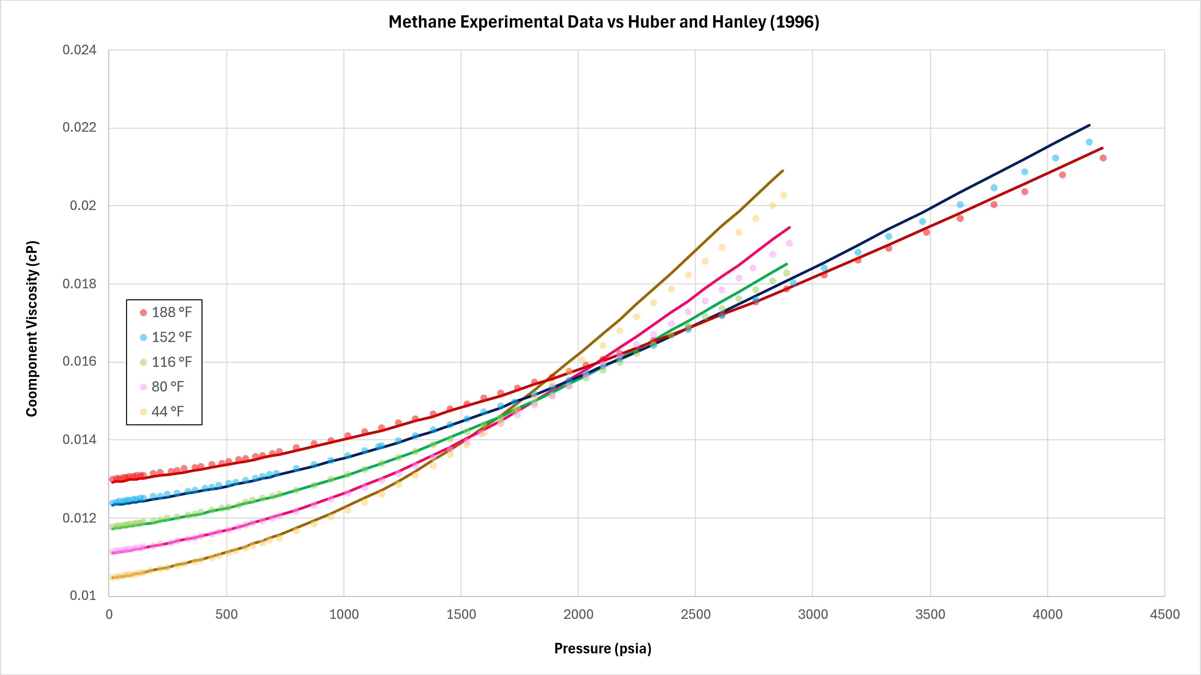
Data for methane at different temperature and pressure published by Schley et al (2004) has been compared against the implemented TRAPP method as detailed in this blog post.
It can be seen that the predictive quality is good within the pressure range modelled. Further modelling should be undertaken to examine the range of performance for the TRAPP method with pure fluids across a wider range of fluids.
Binary Mixtures
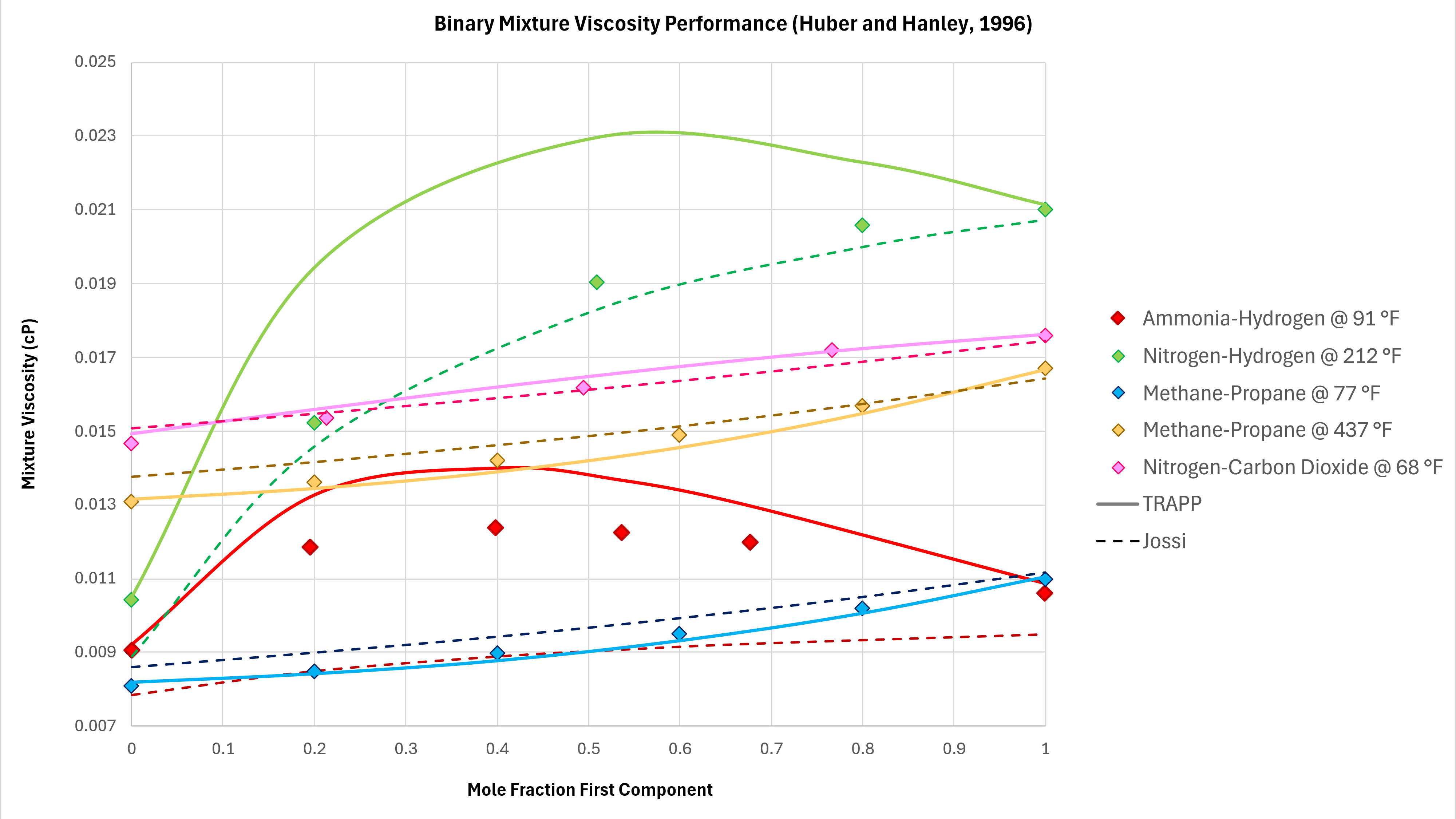
Binary mixtures can exhibit unexpected behaviours. In moving from 100% mole fraction of one component in a binary mixture to the other, the viscosity does not always follow a monotonic trend. That is to say, the viscosity can increase and then decrease, and vice versa. Various binary mixture measured viscosity data is compared against the implemented TRAPP method using data taken from Poling et al (2004) as shown in Figure 3 below. All data is measured at atmospheric pressure.
The TRAPP method is able to capture the non-monotonic behaviour of the Ammonia-Hydrogen binary mixture, and has reasonable predictive capability for Methane-Propane at different temperatures. The prediction of the methane-propane binary mixtures is superior to that of the Lucas method.
As a comparison the Jossi, Stiel and Thodos (JST) method (as used in Lohrenz-Bray-Clark) is also shown on these charts. Generally, with the exception of the Nitrogen-Hydrogen binary pair, the TRAPP method is similar to or outperforms the JST method.
Hydrocarbon mixtures
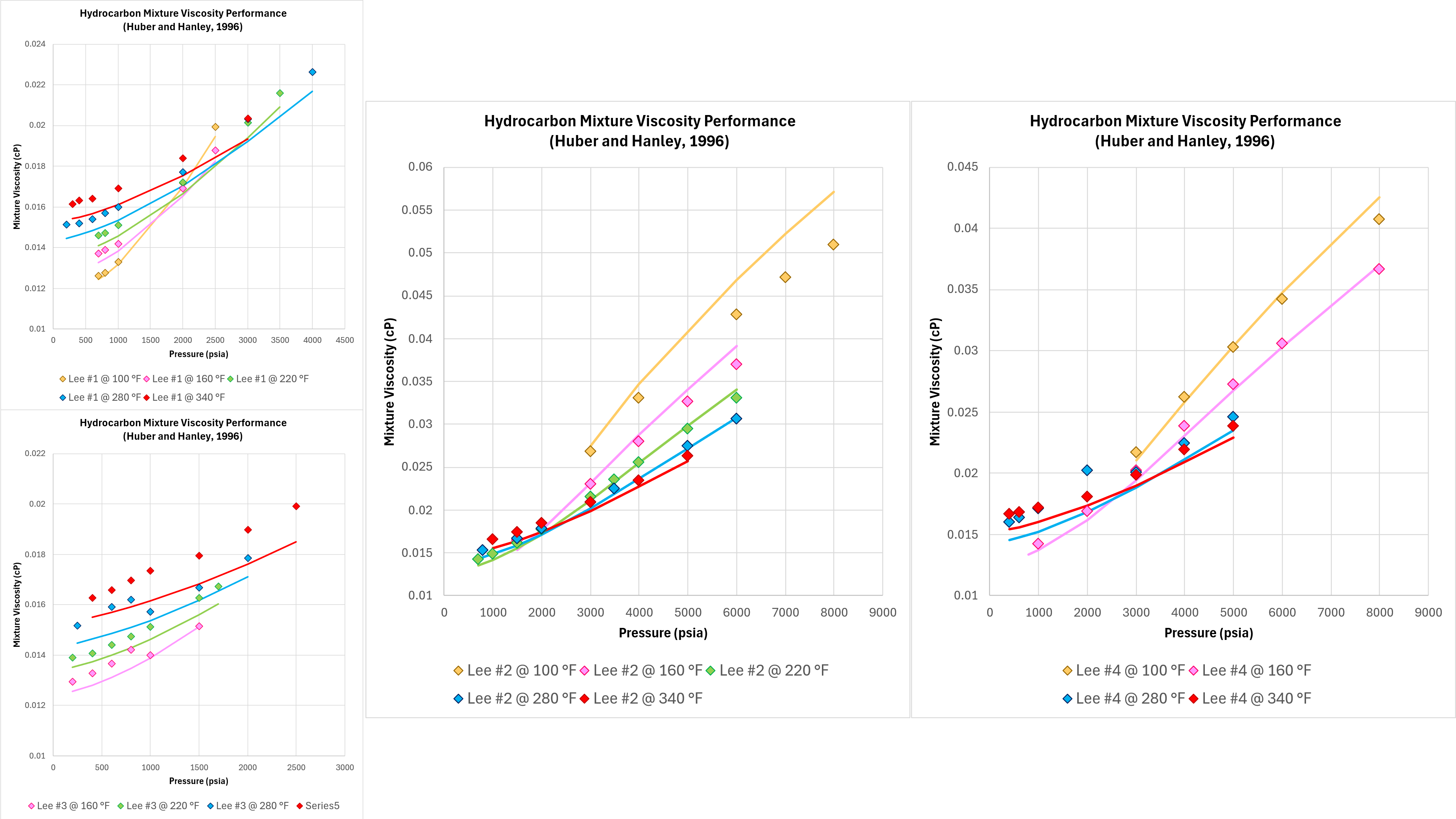
Good performance with pure components and binary mixtures means nothing if the technique does not work on real-world fluids. Four different hydrocarbon gas mixtures and measurements of viscosity were published by Lee, Gonzalez and Eakin (1966). Whilst there are some apparent discontinuities in the measured data, this dataset is sufficient to assess the predictive performance of the implemented TRAPP method as shown in Figure 5 below.
It can be seen that the Lucas method is able to model the correct trends in terms of the viscosity variation with temperature and pressure, and the absolute viscosity predicted is close to the measured values. The accuracy in all cases is superior to that observed with the Chung et al method.
References
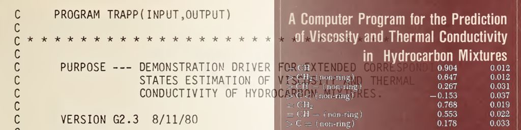
- Ely, J. F. and Hanley, H. J. M. 1981. A Computer Program for the Prediction of Viscosity and Thermal Conductivity in Hydrocarbon Mixtures. NBS Technical Note 1039, National Bureau of Standards. Boulder, Colorado (April 1981). https://doi.org/10.6028/NBS.TN.1039.
- Hanley, H. J. M. 1976. Prediction of the Viscosity and Thermal Conductivity Coefficients of Mixtures. Cryogenics 16 (11): 643-651. https://doi.org/10.1016/0011-2275(76)90035-7.
- Herning, F. and Zipperer, L. 1936. Beitrag zur Berechnung der Zähigkeit Technischer Gasgemische aus den Zähigkeitswerten der Einzelbestandteile (Calculation of the Viscosity of Technical Gas Mixtures from Viscosity of the individual Gases), Gas und Wasserfach 79: 49–54, 69-73.
- Huber, M. L. and Hanley H. J. M. 1996. The Corresponding-States Principle: Dense Fluids. In Transport Properties of Fluids, Their Correlation, Prediction and Estimation, ed. J. Millat, J. H. Dymond, and C. A. Nieto de Castro, Chap. 12, 283-295. Cambridge: Cambridge University Press. https://doi.org/10.1017/CBO9780511529603.
- Lee, A. L., Gonzalez, M. H., and Eakin, B. E. 1966. The Viscosity of Natural Gas. J Pet Technol 18 (8): 997-1000. SPE-1340-PA. https://doi.org/10.2118/1340-PA.
- Poling, B. E., Prausnitz, J. M., and O’Connell, J. P. 2004. The Properties of Gases and Liquids, fifth edition. New York: McGraw-Hill Book Co.
- Reichenberg, D. 1975. New Methods for the Estimation of the Viscosity Coefficients of Pure Gases at Moderate Pressures (with Particular Reference to Organic Vapors). AIChE Journal 21 (1): 181-183. https://doi.org/10.1002/aic.690210130.
- Reichenberg, D. 1977. New Simplified Methods for the Estimation of the Viscosities of Gas Mixtures at Moderate Pressure. Chem 53, National Physical Laboratory, Teddington, England (May 1977).
- Younglove, B. A. and Ely, J. F. 1987. Thermophysical Properties of Fluids. II. Methane, Ethane, Propane, Isobutane, and Normal Butane. J Phys Chem Ref Data 16 (4): 577-798. https://doi.org/10.1063/1.555785.