Generating a series of vertical lift performance curves for input to a reservoir simulator is a difficult task. The data contained in the input keywords form what is known as a lookup table (LUT). The rationale for using this is that computation of the relationship between flowing bottom hole pressure and flowing tubing head pressure is an expensive operation. There are multiple calculations required and repeated requests to compute these values will inevitable consume a large amount of available CPU cycles. The approach used by Pyrus to perform the calculations is described in a post on wellbore simulation.
Since the reservoir fluids are fixed (more or less), the wellbore configuration and tubing diameter does not change, and there is a predictable relationship as pressures increase or decrease, it is more efficient to calculate the pressure relationships once and then interpolate values from these pre-calculated points.
The VFPPROD and VFPINJ Keywords
Reservoir simulators based on the ECLIPSE input deck language use the VFPPROD and VFPINJ keywords. These keywords define the bottom hole pressure necessary to flow along the wellbore for the fluids in question. As can be seen in the help description for the VFPPROD keyword in Figure 1, there are a number of different permutations that can be specified. These include:
- Production Rate: Range of different production rates for which BHP is calculated for every possible permutation.
- Tubing Head Pressure: Range of different THP against which the well must flow.
- Water Flow Ratio: Range of different water flow ratios (exact ratio depends on type of fluid flow) that is used to infer the flow rate of water.
- Gas Flow Ratio: Range of different gas flow ratios (exact ratio depends on type of fluid flow) that is used to infer the flow rate of gas.
- Artificial Lift Quantity: Range of different artificial lift values that can be used to specify the effect of different articial lift schemes on the well flowing performance.
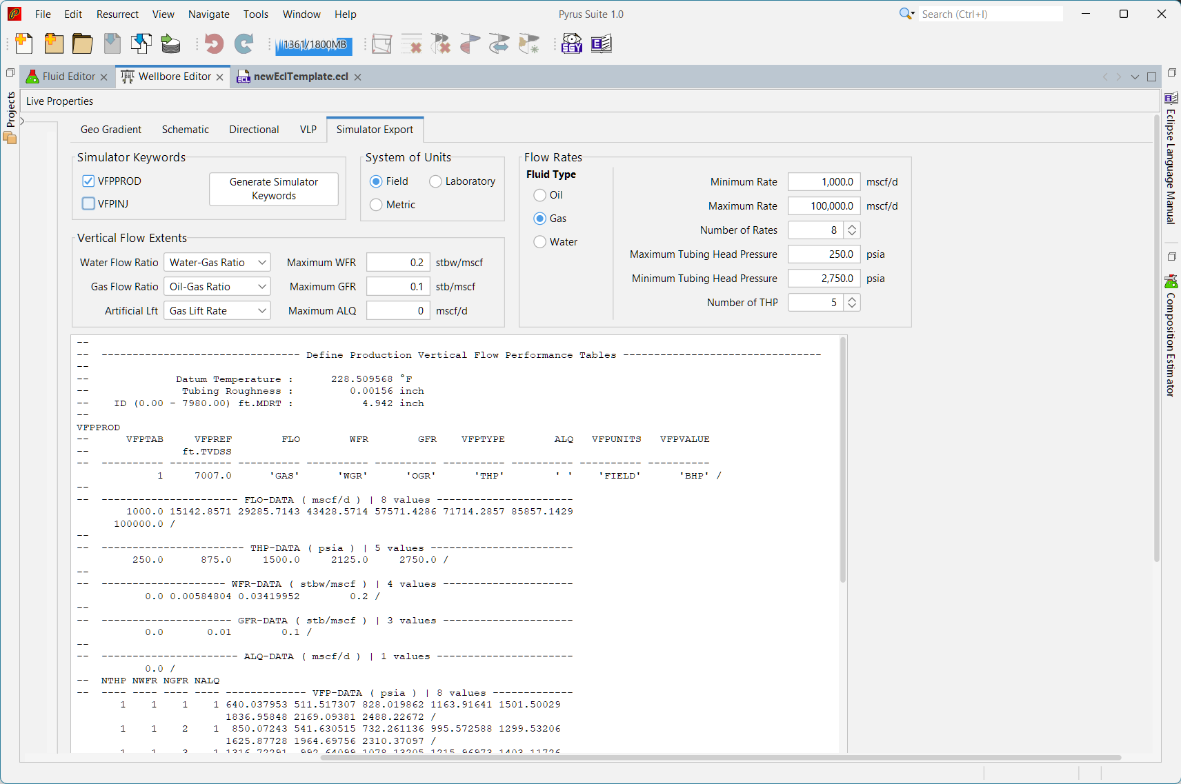
In Figure 1 below there are eight (8) production rates, five (5) tubing head pressures, four (4) water flow ratios, three (3) gas flow ratios and one (1) artificial lift quantity. This gives a total of 8 × 5 × 4 × 3 × 1 = 480 permutations for BHP that must be calculated.
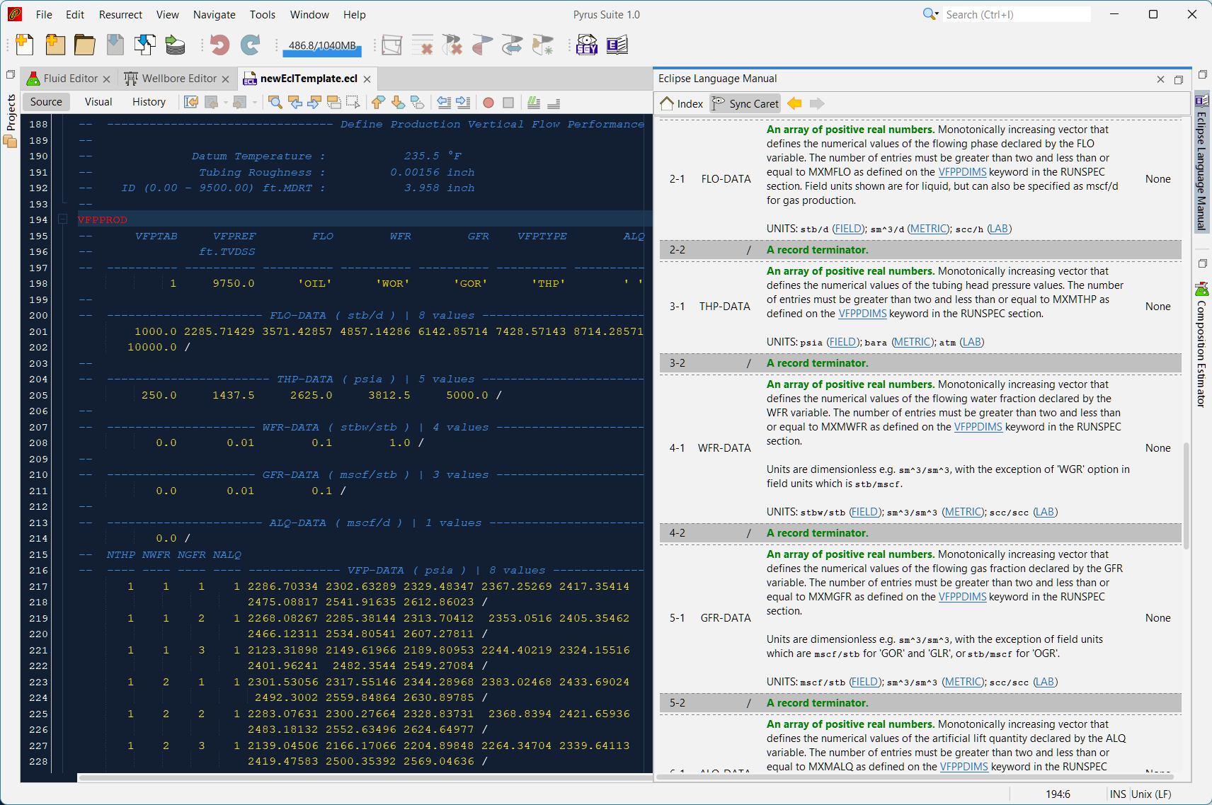
It is the sheer number of calculations that must be determined that makes this keyword a challenge to put together by hand.
Pyrus makes this easy by determining the values to use for each input variable between a user-designated minimum and maximum value, computing the BHP for each permutation, and finally assembling all the results into a neatly formatted keyword that is compatible with the ECLIPSE reservoir simulation language.
Create the Wellbore Description
A conventional wellbore environment comprises a series of concentric holes of decreasing diameter, casing (or liner) strings that are cemented in place within the hole, and a production tubing string up which fluids will flow. Other wellbore environments such as annular flow etc. are possible, but won’t be considered in this basic example.
To define the wellbore we create a new wellbore using the /File/Create/Wellbore menu item.
This opens a wellbore editor, within which we can define the following:
- Location: Elevation of rotary table and ground level, plus definition of the geothermal gradient.
- Trajectory: Wellbore path. If directional data is available, then it can be cut and pasted into the trajectory table. If not, a wellbore trajectory can be generated based on provided targets. Note that the generated trajectory takes into consideration maximum build-up rates that can be achieved and is thus close to real wellbore trajectories. Generally the wellbore path is considered to be a two-dimensional plane in Pyrus e.g., single azimuth. This is because the trigonometry to relate measured depth, vertical depth, inclination, and offset is much more complex than meets the eye.
- Hole Size: Bit sizes used to drill to different measured depths.
- Casing: Casing sizes cemented into the wellbore. Both casing (run to surface) and liner (installed on a liner hanger at a specific depth) can be defined. Pyrus allows wall thickness for casing to be estimated from casing weight in pound per foot (where known). These values are close to those that would be obtained from tubular datasheets provided by OCTG vendors.
- Tubing: Similar to casing, the tubing string can be defined. This does not have to be a single component, although for modelling purposes it is typically simpler to use a single string of uniform inner diameter.
- Completion: Mid-perforations depth and tubing roughness. The perforations depth defines the point at which fluid flow commences in the wellbore, and flow is based on the casing and tubing diameters between this depth and the surface.
Visualise Wellbore
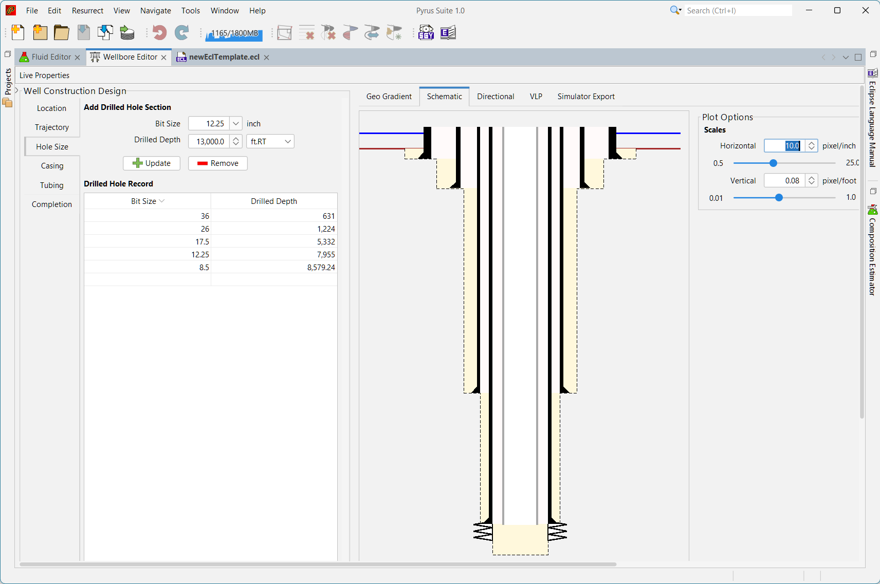
As an example of what type of wellbore can be defined in Pyrus, a similar wellbore to the Pasca A4(AD-1) well drilled in Papua New Guinea by Twinza Oil has been entered into Pyrus. The ‘Geo Gradient’, ‘Schematic’ and ‘Directional’ tabs allow the geothermal gradient, wellbore configuration and trajectory to be visualised.
The well schematic example is shown in Figure 2. This illustrates the hole sizes, casing string and tubulars that have been entered, along with the ground level (seabed in this case), mean sea level and midpoint perforations depth. As Pyrus continues to be developed, the options for more nuanced wellbore illustrations will be added, including:
- Cement
- Packers
- Liner hangers
- Slotted liner
- Gas lift points
- Annotated depths for MDRT and TVDSS
- Fluid flow paths
For the moment the illustration is sufficient to confirm that the wellbore is entered correctly. Note that the wellbore entry does affect the flowing profile calculations. This is because the thermal U-values used in the calculations are determined from the wellbore configuration.
Link to Fluid and Test
To generate a vertical flow profile, we need to know what fluid is flowing in the wellbore. This is defined using the Pyrus Fluid Editor. Typically the Fluid Editor will auto-generate a unique name to identify each fluid, although this can be overridden. Pyrus allows any fluid that has been defined to be used as the primary fluid.
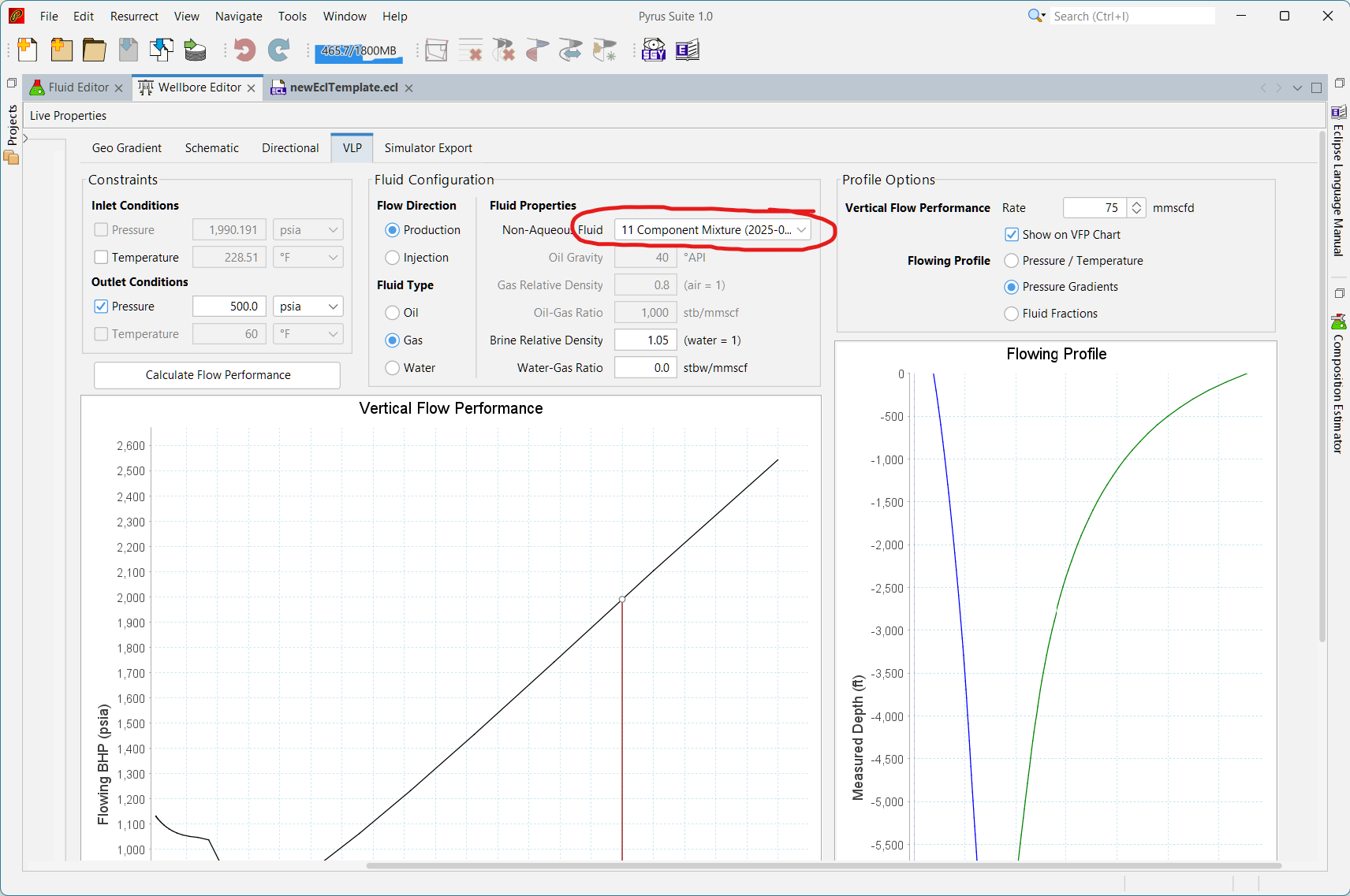
Note that in this context, the gas and oil flowing into the inlet of the tubing are at inlet conditions. The oil will very likely contain solution gas and the gas could contain vaporised oil (condensate). The solution gas and vaporised oil are not included in the determination of oil-gas ratio or gas-oil ratio. Instead these ratios refer to the reservoir oil and gas phases that enter the tubing inlet. For example, above dewpoint the fluid flow entering the wellbore should be 100% gas and no oil. Below the dewpoint, where condensate dropout has occurred and their is sufficient saturation that the oil is mobile, then there will be both gas and oil phases flowing into the wellbore.
In Figure 3 below, a gas production well using the Pasca A4(AD-1) wellbore configuration, and a gas-condensate fluid containing 11 components has been used to create a vertical flow performance curve for a fixed tubing head pressure of 500 psia. Once calculated, the flowing profile along the wellbore can be inspected for a given production rate. In this case, the pressure gradients (hydrostatic in blue and frictional in green) are shown for a production rate of 75 mmscfd.
Simulator Export
This tab is used to create reservoir simulator keywords (currently in ECLIPSE-compatible style) that define the relationships for relative permeability and capillary pressure in each grid block. These keywords can be directly pasted into your simulation software, ensuring a smooth transition from the Rock Matrix Editor to your simulator.
The keywords are generated using the following steps:
- Select Keywords: There are three primary keywords you can generate:
VFPPROD(Vertical Flow Production Table)VFPINJ(Vertical Flow Injection Table) Each of these keywords represents different fluid saturation functions and can be used to model the behavior of fluids in your reservoir.
- Choose Units: By default, the tool uses field units, but you can switch to metric or laboratory units based on your project requirements. This flexibility ensures that your data is accurately represented in the simulation environment.
- Define Fluid: It is necessary to select the primary fluid that will be flowing into the wellbore: oil, gas or water. Depending on the fluid specified, the rates of the other two phases are determined from the water flow ratio and gas flow ratios that are supplied.
- Select Ranges: The ease with which vertical flow tables can be generated means that there can be a temptation to generate a higher resolution of data for the tables. This rarely improves accuracy of calculations or improves simulation speed. On the other hand, excessive resolution can lead to problems with tables where there are ‘overlapping’ curves. Generally the aim should be to ensure that the rates and tubing head pressures cover the anticipated range of possible values for the field, and to use the minimum number of points to describe the variation in behaviour.
- Export: Once you’ve selected the appropriate settings, click the “Generate Simulator Keywords” button. The tool will create the corresponding keywords in the text area below. These are compatible with ECLIPSE and other related simulation software such as OPM-Flow.
- Copy and Paste: Simply copy the generated tables and paste them into your simulator. This direct integration minimizes errors and saves time, making it easier to implement your models.
An example VFPPROD keyword generated using our example Pasca A4(AD-1) wellbore and the gas-condensate fluid is shown in Figure 4 below. This generates a lookup table based on gas rates between 1,000 mscfd to 100,000 mscfd, tubing head pressure between 250 psia to 2,750 psia, maximum water-gas ratio of 0.2 stbw/mscf and maximum oil (condensate) production rate of 0.1 stb/mscf.