Over several decades the oil and gas industry has developed a wide range of correlations that are still regularly used to predict fluid properties based on high level measured characteristics such as API gravity and gas-oil ratios. In many cases, the use of these correlations is a case of near-enough is good enough, but in other cases the predictions turn out to be unreliable. What is really needed is a way to determine fluid properties based on a detailed description of the fluid composition. This is the purpose of an “equation of state” (EOS) and there are many approaches that have been proposed and implemented.
Formulations for predicting fluid properties using an EOS go back over a century and given that this is a field with utility to many industries, not just the oil and gas industry, it is unsurprising to learn that this has been the focus of intense research efforts. Despite this, a definitive EOS that accurately describes the fluid properties of any arbitrary fluid mixture, does not exist. In oil and gas it is common to use one of the variants of what is referred to as a “cubic equation of state”. The EOS implementation used in Pyrus is a combination of the predictive Peng-Robinson formulation (an explanation as to how cubic equations of state are implemented in Pyrus is described elsewhere) for mixtures and the CoolProp library for single pure fluids. This article is focused on the features of the PVT tool itself and how to use it.
Launching the PVT Tool
A version of the PVT tool can be launched using the Tools / PVT / PVT Phase Envelope menu found at the top of the application window. This will open up a separate dialog window that allows for quick testing of properties associated with different fluids. This separate window is modal, meaning that interaction with the main Pyrus application window is not possible whilst this modal dialog window is open. This is intentional as it is expected that the tool is used in a standalone fashion. Note that this standalone tool does not allow the saving of any results. It is purely a utility tool.
Upon opening the PVT tool, the default composition has been set to 100% methane and a simple pressure-temperature (P-T) plot of the phase envelope is shown. The tool allows different compositions to be entered and the results to be visualised in a few different ways, including generation of suitable keywords in ECLIPSE language format for import into a reservoir simulator.
Using the PVT Tool
The PVT tool can appear a little daunting at first as much of the functionality can be directly accessed from the dialog window that opens up. This is a deliberate design choice. Hiding much of the functionality behind other tabs or options provides a cleaner and less busy interface, but the trade-off is that it requires more clicks and / or keypresses to use the tool. Thus the interface actually gets in the way and the tool loses any benefits of being quick and functional.
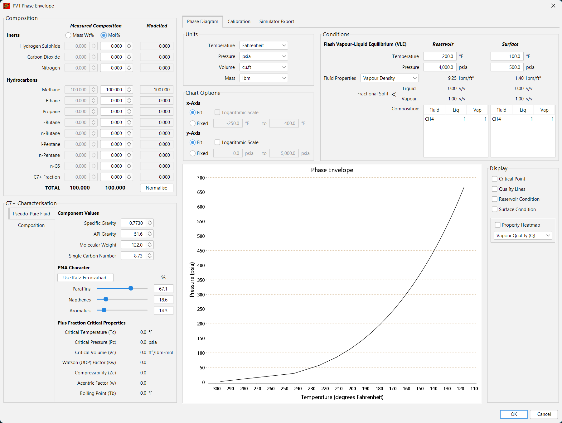
The tool is structured into several areas as shown in the screenshot below:
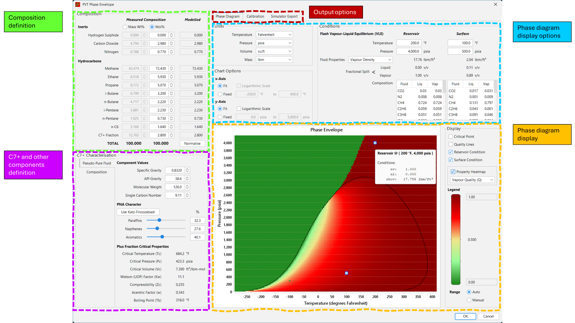
The purpose of each area is as follows:
- Composition Definition: The high level composition of the mixture can be entered here, either using the molar or mass weight percentage composition. The components shown are those typically encountered with hydrocarbon mixtures. Other components can be entered using the C7+ component definition (in which case it the C7+ component is just an ‘other’ bucket to capture a more detailed compositional definition using other components).
- C7+ Characterisation: This is where the properties for the C7+ fraction are defined. The default approach used is for a single C7+ pseudo-pure fluid to be defined. This is a single component that represents the entire C7+ fraction. The tool will calculate the properties for the pseudo-pure fluid automatically based on the provided specific gravity, density, molecular weight, single carbon number and paraffin-naphthene-aromatic (PNA) ratios. Alternatively a more detailed composition can be defined for the heavy fraction, using multiple components as opposed to a single pseudo-pure fluid.
- Output Options: Different tabs allows switching between different output formats and options. The default
Phase Diagramtab provides for display of a phase envelope. There are many different options that can be set to control the visualisation of the generated envelope. Other tabs includeCalibrationwhich allows a different cubic EOS to be used, or tuning of the current EOS to be implmented, andSimulator Exportwhich generates keywords describing the fluid that can be imported into an ECLIPSE simulation deck. - Phase Diagram Display Options: Sets the visualisation options for the phase envelope display. This includes the choice of units, axis scales, superposition of two different ‘reservoir’ and ‘surface’ conditions onto the phase envelope and the associated properties and compositions at these conditions, and option display of a background ‘heatmap’ which shows how a selected property varies over the phase envelope.
- Phase Diagram Display: This is the phase envelope for the mixture, showing the boundary between the single phase and two-phase regions.
The tool presents ‘live’ results. So every time a change is made to the inputs, the outputs are updated to reflect the current input state. This means the tool is powerful with respect to illustrating what effect small changes can have on the overall phase envelope.
Entering Compositions
The tool requires that a detailed composition of the mixture is known. It is not possible to estimate compositions from high level fluid measurements such as specific gravity and gas-oil ratios using this tool.
Most compositions provided by laboratory analysis will show similar components to those in the ‘Composition’ panel of the tool. Values should be entered into the spinner for each component as percentages e.g., 100% is entered as 100.000. To enter a value, simply type into the spinner and either use ENTER or TAB to commit the value entered. The difference is that ENTER will simply end editing of the value and enter it into the composition, whereas TAB will enter the value being edited into the composition and then jump to the next component’s value spinner and select all the text. This allows compositions to be entered very quickly. Simply type the value, hit TAB, type the next value, hit TAB, and so on…
Alternatively, it is possible to tweak values already entered using the spinner up and down arrows. These will increment and decrement the value respectively by 1%. This function is useful to visualise the sensitivity of the composition to a particular component. Even if the original composition that has been entered adds to 100%, by tweaking a single component it can be observed that the modelled composition is automatically normalised so that this adds up to 100%. The Normalise button will commit this modelled composition to the values being entered (and thus replace the original values) if desired.
Cut and Paste From Spreadsheet
It is also possible to copy and paste compositions from a spreadsheet into the Pyrus PVT tool. To copy from a spreadsheet the composition data must be set up as two columns, with the first column containing the components and the second column containing the mol% fractions. The units for the fractions can be either percentage or fraction (v/v) as long as they are consistent. The main components (up to C11) are:
| Component Code | Description |
|---|---|
| CO2 | Carbon Dioxide |
| N2 | Nitrogen |
| H2S | Hydrogen Sulphide |
| CH4 | Methane |
| C2H6 | Ethane |
| C3H8 | Propane |
| IC4 | iso-Butane |
| NC4 | n-Butane |
| IC5 | iso-Propane |
| NC5 | n-Propane |
| C6 | Hexane Fraction |
| C7+ | Heptanes Plus Fraction |
| NC7 | n-Heptane |
| NC8 | n-Octane |
| NC9 | n-Nonane |
| M-Cy-C6 | MethylCycloHexane |
| C7H8 | Toluene |
| C8H10 | EthylBenzene |
| O-X | Ortho-Xylene |
| M-X | Meta-Xylene |
| P-X | Para-Xylene |
| TriM-B | TriMethylBenzene |
| C10 | C10 Fraction |
| C11 | C11 Fraction |
Other component codes can be seen in the compositional list in the tool itself.
Specifying C7+ Fraction
The C7+ fraction can be specified either as a single pseudo-pure fluid component, or through entering a more detailed composition for the heavier components. The computation time increases as more components are included in the compositional description. However, unlike in a compositional simulation which is required to perform flash calculations for the EOS on potentially millions of cells, there are comparatively fewer flash calculations that take place when running the tool. Running a highly detailed compositional analysis should not be prohibitive.
On the other hand, the properties of heavier fractions can influence the tuning for equation of state. More control over the tuning is possible by tweaking the properties of a composition with just a single C7+ fraction in comparison to a detailed compositional description. Lumping heavier components into a single C7+ fraction can therefore be advantageous both in terms of computational speed and flexibility.
Entering a Pseudo-Pure Fluid Component
A single pseudo-pure fluid component for the C7+ fraction can be defined in the Pseudo-Pure Fluid tab of the ‘C7+ Characterisation’ panel. The component properties such as the critical temperature, pressure and volume are all determined via correlations, with care taken that the mass, specific gravity, single carbon number and PNA distribution remain consistent.
Typically laboratory reports will report the molecular weight and density (specific gravity) of the C7+ fraction. These two parameters are the minimum that need to be entered to change the properties of the C7+ fraction. The molecular weight, single carbon number, PNA distribution and critical properties are all calculated automatically as any of these input values are altered.
It is important to note that the C7+ fraction contains many different compounds, and that the distribution of paraffinic, napthenic and aromatic compounds changes the relationship between the density and the molecular weight. Often, the reported molecular weight is based on an assumption that the heavier C7+ components have properties that align to the published Katz-Firoozabadi single carbon number compounds. Whilst there is nothing inherently wrong with such an approach, it should be remembered that this is an assumption. Thus, in comparison to the specific gravity (which is usually measured and thus reasonably well defined), the molecular weight and PNA distribution are more uncertain and can be adjusted as necessary to tune the EOS.
When cutting and pasting a C7+ component into the Pyrus PVT tool, there are two special component codes that are used to indicate the molecular weight and density (specific gravity) of the C7+ fraction:
| Component Code | Description |
|---|---|
| C7+MW | Heptanes Plus Molecular Weight |
| C7+GAMMA | Heptanes Plus Specific Gravity (relative to water = 1) |
Entering a Detailed Composition for Heavy Components
A more detailed description of the heavy fractions can be entered by selecting the Composition tab of the ‘C7+ Characterisation’ panel. By default the Define C7+ Fraction Components checkbox is not selected, and the composition shown is either blank in the case that there is 0.0% C7+ Fraction in the composition, or shows seven hypothetical components which are created by splitting the defined C7+ Fraction. For more explanation concerning why it is beneficial to split the C7+ component into several components, see the description for the calibration and settings section.
By selecting the Define C7+ Fraction Components checkbox, a table of possible additional components is shown. Notice that the C7+ Fraction in the ‘Composition’ panel is disabled when this is selected. Entering Mass Wt% or Mol% values for each component will automatically update the C7+ Fraction shown in the ‘Composition’ panel. Furthermore, if the Pseudo-Pure Fluid tab of the ‘C7+ Characterisation’ panel is selected after entering several detailed components, it can be seen that although the inputs for the pseudo-pure fluid are also disabled, these update to reflect the approximate properties for the detailed composition that has been entered.
Shown below is an example use of the detailed composition to show the phase envelope for 95% carbon dioxide plus contamination with 5% air. The 5% air is entered as a component in the C7+ Fraction, meaning the overall composition is 95% carbon dioxide and 5% air.
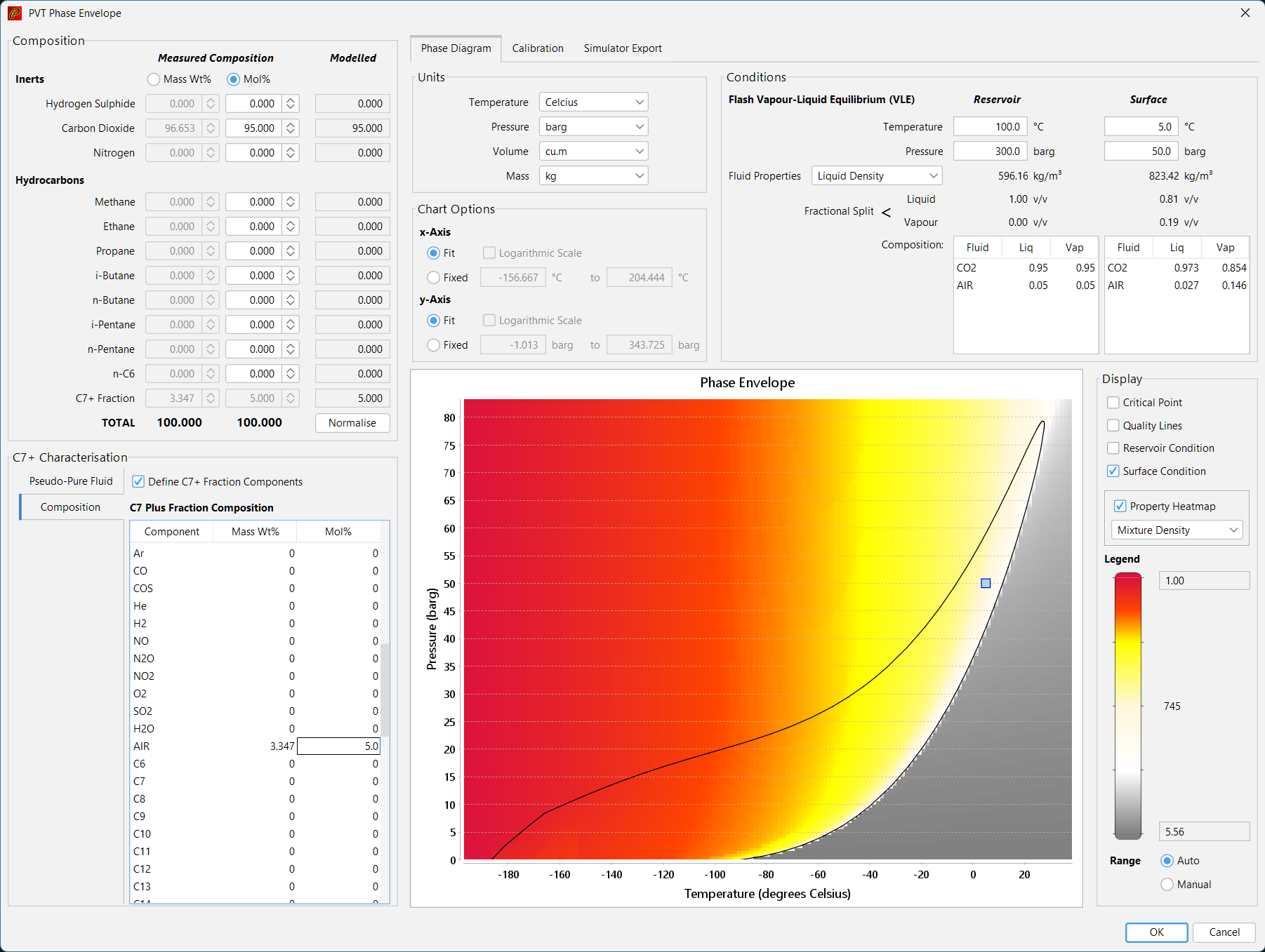
There are only a limited selection of compounds available and it is not possible to define custom components to include in the detailed composition. The tool is designed to be a simple and easy to use tool for quickly accessing results, rather than a comprehensive swiss army knife. The compounds included are:
- Straight chain alkanes: Unbranched normal paraffins with carbon numbers from 7 to 20.
- Common isomers: Common branched paraffins, naphthenes and aromatic isomers for single carbon numbers between 5 and 8.
- Other non-hydrocarbon gases: Hydrogen, oxygen, water and air (as a pseudo-pure fluid).
- Katz-Firoozabadi single carbon number fractions: All KF SCN components from C6 to C50.
Output Formats
The tabs in the upper central portion of the PVT tool control what output from the equation of state is produced. The output options are:
- Phase Diagram: Displays a phase envelope of the composition on a chart plot. There are various options available that govern how the phase envelope is displayed.
- Calibration: Allows a different cubic equation of state to be applied, toggles C7+ fraction splitting on or off, and controls tuning of key cubic equation parameters. It is possible to enter results from laboratory tests to assist with matching the equation of state model performance against measured results.
- Simulator Export: Generates keywords based on this composition for the ECLIPSE simulator.
Displaying the Phase Envelope
The display of the phase envelope is the default output panel option for the PVT tool. It is not necessary to select this in order to view the phase envelope, unless a different output panel has previously been selected.
There are a range of options available for controlling the display of the phase envelope. Unlike many charting applications where these options are typically hidden from the user, the PVT tool deliberately exposes controls for the choice of display units and the axes scales in controls placed above the phase diagram itself. This improves the ease with which the desired display for the chart plot can be achieved through ensuring rapid visual feedback.
In addition there are two reference conditions that can be superimposed onto the plot of the phase envelope. Notionally these are identified as a reservoir and surface condition, but these can be repurposed for any other two conditions if desired. For each of the two conditions, the resulting liquid-vapour equilibrium split is shown, along with the composition for the liquid and vapour fractions. A single fluid property can also be shown.
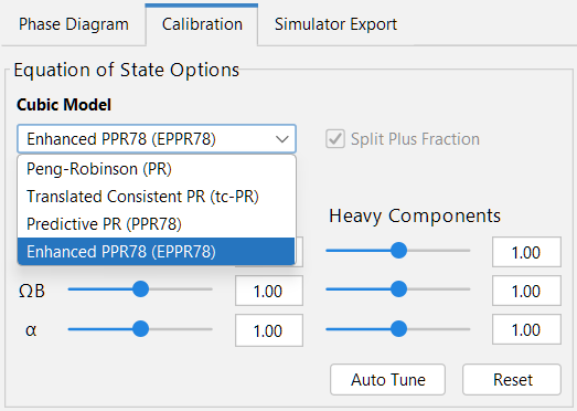
Calibration and Settings for Equation of State
The choice of cubic equation of state and options related to how the cubic EOS is implemented can be set from the Calibration tab. The choice of cubic EOS is selected using the drop-down menu as shown in the figure below. The PVT tool in the Pyrus Suite supports the Peng-Robinson EOS, and three variations of the predictive Peng-Robinson EOS which are essentially state-of-the-art with respect to cubic equations of state as at the time that this part of Pyrus was originally written (the date stamp in the source code reveals I started writing the cubic equation of state class on 7 March 2018).
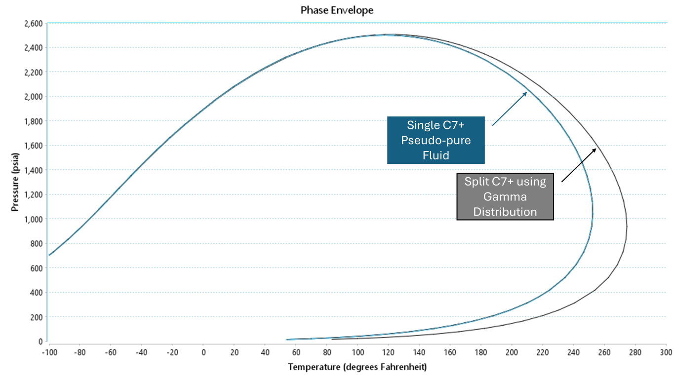
If the C7+ Fraction is defined using a single pseudo-pure fluid, then the default option is to split the single component into seven fractions using a gamma distribution model. The aggregate split fractions have the same overall properties as the single pseudo-pure fluid. However, the inclusion of heavier molecular weight components influences the phase envelope and thus the inclusion of split components from the C7+ Fraction is recommended. This can be seen in the comparison below where the use of spitting results in the cricondentherm being pushed to the right.
Simulator Export
Generation of ECLIPSE keywords PVDO, PVDG, PVTO and PVTG can be accomplished via the Simulator Export tab. The reservoir condition that is set on the Phase Diagram tab is used to assign the reservoir temperature used as the basis for the keywords. Depending on the fluid composition that is defined the live oil (containing dissolved gas) and live gas (containing condensate) options may be disabled.
Generate the keywords using the Generate Simulator Keywords button. This will create the keywords in the text area below the controls. The text that was generated can be copied from this text area using keyboard shortcuts CTRL + A to select all the text, followed by CTRL + C to copy the text to the operating system clipboard.
Setting Display Options for Phase Envelope
The display of the phase envelope is determined using this section of the tool. There are four different aspects that can be controlled in the Phase Diagram tab.
- Units: Sets the units used for input and display of temperature, pressure, volume and mass.
- Chart Options: Sets the scale range used for the x- and y- axes.
- Conditions: Defines the conditions to be optionally displayed on the chart, and sets display options such as inclusion of a heatmap to show variation in properties over the range of values for the displayed chart area.
- Chart Plot Area: Displays the chart itself and allows zooming, copying or saving of the image to file.
Units
The units used for entering and displaying results are set using the dropdown boxes for each quantity. It is entirely possible to mix imperial and metric units. Whether or not this is advisable is debatable, but there are occasions where this level of flexibility could be useful.
Note that temperature can be shown both in absolute scale (Rankine and Kelvin) or conventional scale (Fahrenheit and Celsius). Pressure can be shown as either absolute atmospheric e.g., zero is no pressure, or gauge e.g., zero is atmospheric pressure = 1.0 atm.
Changing any unit in the relevant drop-down will change the units used for display on the chart axes, all input values and all displayed values. Note that any input values are automatically converted from the previous unit to the new unit.
Changing Axis Range
The default setting for axis ranges is to attempt to choose a range that fits the entire phase envelope. Generally, when inputting data, this is a sensible setting as it ensures that the results of the phase envelope generated for any composition are always visible.
Conditions
Two points can be superimposed onto the phase envelope diagram to indicate a specific temperature and pressure condition. Notionally these are the reservoir and surface conditions, although there is no restriction concerning the values that can be entered for each.
After the temperature and pressure are specified for each point, the checkbox is used to enable the display of the condition point on the phase envelope diagram. Hovering over the displayed point with the cursor will reveal a popup showing the vapour and liquid fractions, and the density at that point. The point can be moved interactively by left-clicking the point and then moving the mouse to a new location. The temperature, pressure and flash properties adjust as the condition point is moved. Left-clicking a second time will end the move action. Note that this is not a click and drag behaviour (a click-move-click action is considered more accurate than a click-drag action).
The single phase or two phase nature of each condition is shown by the fractional split for liquid and vapour. Any selected property can also be shown for each condition. The different properties can be selected via the drop-down menu. All properties are not shown simultaneously.
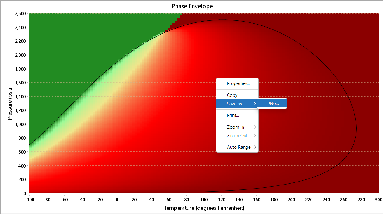
Additional display options can also be set in the ‘Conditions’ panel. These include showing the critical point and / or quality lines (lines of constant vapour or liquid fraction in the two-phase region) on the diagram. A heatmap can also be shown under the phase envelope. This shows a crude variation for the value of the chosen display property of the heatmap. The default property shown is the vapour quality, where 100% vapour is shown as dark red and 100% liquid is shown as green. The heatmap colours transition from red through to green in the two-phase region, depending on the vapour-liquid split.
Interacting with the Phase Envelope
Left-click and dragging to the bottom right will perform an interactive zoom to the selected area. Left-click and drag to the upper left will reset the zoom to the default range for the x-axis and y-axis.
Right-clicking in the plot area for the phase envelope allows the image to saved as a portable network graphics (PNG) image capture, copied or printed.