A common approach to modeling relative permeability curves for input to a reservoir simulator is to match synthetic curves to measured rock data or use the actual measured curves with appropriate smoothing. This measured rock data is obtained from special core analysis (SCAL). However, obtaining a representative sample of core from the reservoir can be challenging, especially in highly heterogeneous formations. To address this, Pyrus has implemented a tool that models the relative permeability curves using fundamental rock data instead of relying solely on SCAL.
The Rock Matrix Editor facilitates modeling rock property relationships, including porosity-permeability and relative permeability curves, for both sandstone and carbonate lithologies. It transforms geological descriptions into estimated property relationships through mathematical models and first principles.
This tool is particularly useful in scenarios where routine and special core analysis results are unavailable, either because the work hasn’t been completed or no hard rock samples are available. Even when rock core samples are collected, the tool helps guide or constrain the rock description. Laboratory measurements often bias towards the more competent parts of the core, making it difficult to take measurements from vuggy carbonate or unconsolidated sand—facies that may have excellent reservoir properties. By using this method, you can create a generalized description of the rock matrix validated by laboratory measurements, rather than basing the entire rock description on a small fragment of rock core (akin to the tail wagging the dog).
Inputting Rock Facies Description
Reference Porosity
There are two different approachs that can be used to create relative permeability tables for different porosities. The first is to assign a different SATNUM value to cells that fall within a specific porosity range. The SATNUM keyword defines the saturation tables (relative permeability and capillary pressure tables) region numbers for each grid cell block. The region number specifies which set of relative permability tables (SGFN, SWFN, SOF2, SOF3, SOF32D, SGOF, SLGOF and SWOF) are used to calculate the relative permeability and capillary pressure in a grid block.
When creating relative permeability tables for different SATNUM cells, you can use different reference porosities.
Alternatively, if you are using endpoint scaling via the ENDSCALE keyword, you can stick with the default of 25% for the reference porosity. This requires endpoints to be entered for each cell (easily achieved in Pyrus via generation of OPERATE keywords) and the input curves are then fit to match the provided endpoints.
Of course, if there are different facies, it is possible to assign different SATNUM values for each facies type and combine this with endpoint scaling to handle the differences in porosity for each of those facies types. This is my preferred approach.
Theoretical Pore Channel Model
The porosity-permeability and relative permeability curves are fundamentally driven by the pore geometry, utilizing a theoretical pore channel model constructed by Müller-Huber, Schön, & Börner (2015). This model is a modification of the simple capillary tube model and includes a variable pore radius. The pore throat radius (rt) is defined at the narrow end of the channel, which then increases to a radius (rb) at the pore body.
Rather than requiring input in terms of both pore body and pore throat sizes, the rock matrix editor uses the cementation exponent (m) and the pore body radius. This is because the cementation exponent is related to tortuosity of the flow path through the rock matrix, and can be related to the pore body to pore throat ratio (rb/rt). An overview of the rock model used is explained elsewhere in this blog. Cementation exponent is familiar to petrophysicists and reservoir engineers as it is used in Archie’s equation.
Cementation exponent and pore body diameter can be obtained from special core analysis or estimated based on geological assessment input. Where these values are hard to estimate or not otherwise available, they can instead be generated via a description of the rock fabric. Pyrus has in-built models that predict the cementation exponent and pore body diameter for sandstone and carbonate based on a description of the rock fabric.
Sandstone Lithologies
For sandstone, simply input the average grain size and the degree of sorting. These parameters tweak the pore body diameter and cementation exponent, giving you more accurate permeability and relative permeability curves.
- Grain Size: This is the average grain size of the sandstone, measured in millimeters. The grain size directly influences the pore geometry. Larger grains typically indicate higher permeability because of the larger pore spaces between the grains. Input the grain size value to define the characteristic dimensions of the pore spaces. Pyrus allows the input of grain sizes from very fine sand through to very fine pebbles. The grain sizes used by geologists are: 1. Clay: Less than 0.004 mm 2. Silt: 0.004 to 0.0625 mm 3. Sand: - Very Fine Sand: 0.0625 to 0.125 mm - Fine Sand: 0.125 to 0.25 mm - Medium Sand: 0.25 to 0.5 mm - Coarse Sand: 0.5 to 1 mm - Very Coarse Sand: 1 to 2 mm 4. Granule: 2 to 4 mm 5. Pebble: - Very Fine Pebble: 4 to 8 mm - Fine Pebble: 8 to 16 mm - Medium Pebble: 16 to 32 mm - Coarse Pebble: 32 to 64 mm 6. Cobble: 64 to 256 mm 7. Boulder: Greater than 256 mm
- Degree of Sorting: This parameter ranges from 0 to 2.5, where 0 indicates extremely well-sorted sandstone, and 2.5 represents very poorly sorted sandstone. Hovering over the slider should reveal a tooltip that helps to guide the value to be entered for different degrees of sorting. Sorting refers to the distribution of grain sizes within the rock. Well-sorted sandstones have uniform grain sizes, leading to more consistent and predictable pore geometries, whereas poorly sorted sandstones have a mix of grain sizes, resulting in more complex pore geometries. A common statistical method to describe sorting involves using the D25 and D75 grain sizes, where D25 is the grain size below which 25% of the sample’s weight is finer, and D75 is the grain size below which 75% of the sample’s weight is finer. The D75/D25 ratio provides a measure of the spread of grain sizes in the sample. A lower ratio indicates well-sorted sediment, while a higher ratio indicates poorly sorted sediment.
Carbonate Lithologies
Carbonates require a different approach that builds on the classes of carbonates described by Lucia (1995). The carbonate lithology is described in geological terms, noting the dominant rock type, texture, and composition. From this description, a rock fabric number that aligns to Lucia’s carbonate classes is determined. This method aligns with how field geologists describe rocks, ensuring the tool is both intuitive and precise. A comparison of how the rock model can be used to generate porosity-permeability relationships consistent with Lucia’s carbonate classes is described in an analysis post on this blog.
- Lithology Description: Instead of focusing on grain size and sorting like sandstone, carbonate lithologies require a detailed geological description. Identify the dominant rock type (e.g., mudstone, wackestone, packstone, grainstone) to set the stage for further analysis. This classification is crucial as it influences the pore structure and fluid flow characteristics. The value used to describe the ‘muddiness’ of the carbonate fabric.
- Dolomite Crystal Size: This is used as a proxy for the extent of diagenetic effects on the rock texture. Rocks with grain or crystal sizes greater than 100 micrometers (e.g., grainstones, dolograinstones, large crystalline dolostones) typically have high permeability due to their larger pore spaces. Diagenesis can significantly affect the porosity and permeability. If the carbonate is not dolomotised but has been affected by diagenesis, such as dissolution to create vugs, then a large dolomite crystal size should be entered as a proxy for increased porosity and permeability.
Ancillary Parameters
The Endpoints Tab
Key to the modelling process, the Endpoints tab focuses on four main saturation endpoints. These endpoints are modelled consistently using Pyrus’ rock model.
- Irreducible Water Saturation (Swirr): Estimated using the Holmes-Buckles model. The benefits of this model and how it can be tuned to match actual relationships between rock porosity and water saturation are described in the analysis section of this blog. The Holmes-Buckles relationship is based on the classical Buckles equation where porosity times irreducible water saturation is a constant. The equation is modified to introduce a porosity exponent. Holmes indicates that the value of Q can vary between 0.8 to 1.3, and that for many reservoirs a value of Q = 1 i.e., the original Buckles formula, is reasonable. A more significant variable in the equation is the constant, or the Buckles number. Holmes notes that ranges for the constant are:
- Sandstones: 0.02 to 0.10
- Inter-granular carbonates: 0.01 to 0.06
- Vuggy carbonates: 0.005 to 0.06 Typically, the higher the constant, the smaller the average pore throat size within the rock matrix. The relationships for sandstones and carbonates have been devised by considering the recommended Buckles numbers for different rock types and comparing these against typical cementation exponents for those rock types. These relationships are designed to capture the expected behaviour of different rock types. You can manually adjust the C and Q inputs used to generate the Swirr value or input your own Swirr value.
- Residual Gas Saturation after Water Invasion (Sgrw): Estimated with the Holtz model, which generates the maximum trapped gas saturation (Sgtmax) based on porosity. The method proposed by Holtz (2002) modifies the Land equation to produce a relationship that means the residual gas saturation is always equal to or less than the initial gas saturation. The method generates a family of curves depending on the rock quality, with higher porosity rock yielding lower residual gas saturation. Override with your own values if needed.
- Residual Oil Saturation after Water Invasion (Sorw): Here the oil and the displacing fluid are immiscible. For a water-wet rock, whereby water adheres to the rock matrix, the residual oil saturation can be considered to be the same as the residual gas saturation. For an oil-wet rock, where the oil-water contact angle > 90 degrees) we might expect the behaviour of the residual oil to be similar to water as the wetting phase in a water-wet rock i.e. Sorw = Swirr.
- Residual Oil Saturation after Gas Invasion (Sorg): The situation for the residual oil saturation after gas invasion is different. In this scenario we must consider carefully the miscibility between the gas and oil phases. For a gas-condensate above the dewpoint pressure, the oil and gas phases can be considered miscible. Theoretically, at least, all the oil could therefore be displaced meaning the residual oil saturation is zero. On the other hand, at low pressure and temperature the oil and gas become immiscible and the fluids will behave more like the case of oil being displaced by water. In this case the wettability of the rock again becomes an important consideration. Al-Nuaimi et al. (2018) published an interesting approach to modelling the change in Sorg in relation to the interfacial tension (IFT) between gas and oil using a Michaelis Menten Kinetics model. As IFT decreases, the residual oil saturation to gas approaches zero. For the purposes of our model we will simplify the Al-Nuaimi approach and observe that we are simply looking for a reduction in Sorg under miscible conditions. We set σcrit to a fixed value of 0.15 and from this we can determine the miscible Sorg. Again, manual inputs are welcome for either σcrit or Sorg.
The Rock Properties Tab
Two critical parameters define rock properties:
- Wettability: Describes the fluid that adheres to the rock surface via contact angle. The contact angle can have values between 0 and 180 degrees and is used to determine whether the rock is water-wet or oil-wet based on contact angles < 90 degrees = water-wet and > 90 degrees = oil-wet.
- Shape Factor: Ranges from 1 to 3, influencing the curvature of relative permeability curves. Lower permeability rocks have a shape factor closer to 1, and higher permeability rocks closer to 3. Default estimates can be overridden. The shape factor is somewhat arbitrary and can be used to tune the shape of the resulting relative permeability curves if necessary.
The Fluids Tab
Describes fluid properties at reservoir conditions and is used principally to determine the miscibility of gas and oil. The gas-oil interfacial tension is estimated following the method of Abdul-Majeed (2000). This is a reasonable approximation to the Ramey (1973) pseudocompositional black oil approach. For oil with very low gas-oil ratio, this will give a surface tension that is effectively the immiscible value.
- Reservoir Temperature and Pressure: Enter the reservoir conditions.
- Densities of Gas, Oil, and Water: Densities (or pressure gradients) for the fluids encountered in the reservoir.
These parameters calculate gas-oil ratio and interfacial tension, crucial for accurate simulation.
Outputs and Simulator Export
Permeability Charts
There are three chsrts produced. These are:
- Porosity-permeability relationship.
- Water-oil relative permeability.
- Gas-oil relative permeability.
Both drainage and imbibition curves are shown. For the water-oil relative permeabilities, the water relative permeabilities for drainage and imbibition are modelled identically. The oil relative permeabilities are shown in dark green for the drainage curve and light green for the imbibition curve. For the gas-oil relative permeabilities, the oil relative permeabilities for drainage and imbibition are modelled identically. The gas relative permeabilities are shown in dark red for the drainage curve and light red for the imbibition curve.
Charts update in real-time as you adjust inputs, with customizable logarithmic scales. This real-time feedback allows for immediate visualization of how changes in geological descriptions impact the derived rock property relationships. The charts can be exported as portable network graphics (PNG) format image files by right-clicking on the chart and selecting the context menu item Save as > PNG....
Simulator Export
This tab is used to create reservoir simulator keywords (currently in ECLIPSE-compatible style) that define the relationships for relative permeability and capillary pressure in each grid block. These keywords can be directly pasted into your simulation software, ensuring a smooth transition from the Rock Matrix Editor to your simulator.
The keywords are generated using the following steps:
- Select Keywords: There are three primary keywords you can generate:
SWOF(Saturation-Water-Oil Functions)SGOF(Saturation-Gas-Oil Functions)SGWFN(Saturation-Gas-Water Functions) Each of these keywords represents different fluid saturation functions and can be used to model the behavior of fluids in your reservoir.
- Choose Units: By default, the tool uses field units, but you can switch to metric or laboratory units based on your project requirements. This flexibility ensures that your data is accurately represented in the simulation environment.
- Generate Curves: Decide whether you want to generate a single set of curves or separate tables for drainage and imbibition. Typically, you generate a single set for initialization (drainage) and another for production (imbibition). Using two sets of curves allows for a more comprehensive and realistic modeling of fluid flow in the reservoir, particularly in transition zones where the initial gas saturation is less than that which would occur if the water saturation were are irreducible water saturation.
- Export: Once you’ve selected the appropriate settings, click the “Generate Simulator Keywords” button. The tool will create the corresponding keywords in the text area below. These are compatible with ECLIPSE and other related simulation software such as OPM-Flow.
- Copy and Paste: Simply copy the generated tables and paste them into your simulator. This direct integration minimizes errors and saves time, making it easier to implement your models.

