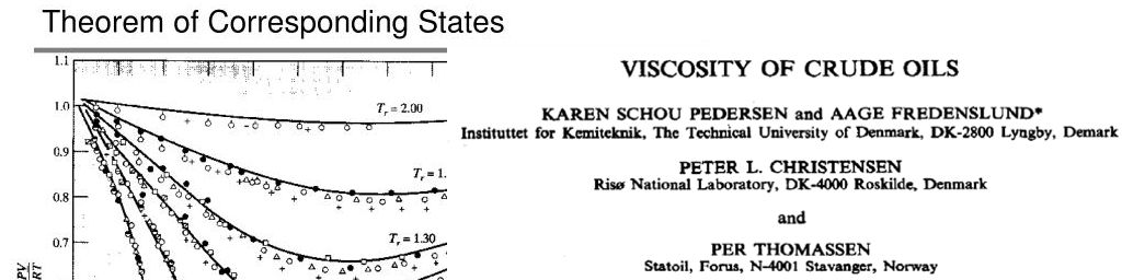
Pedersen et al (1984, 1987) devised a method to calculate viscosity based on the corresponding states principle (CSP). Corresponding states is a recognised principle that should be familiar to most petroleum engineers as it forms the foundation of the classical Z-factor correlation chart first published by Standing and Katz (1942). The general principle is that all components behave similarly in relation to their critical point. Thus by expressing temperature and pressure in terms of reduced temperature (T/Tc) and reduced pressure (p/pc), any component with the same reduced temperature and reduced pressure (a corresponding state) should have the same Z-factor.
Similarly, for a corresponding state of reduced temperature and reduced pressure, any component should have the same reduced viscosity (μ/μc). If we can accurately model the viscosity for a reference component, then we can easily determine the viscosity for any other component, provided the critical point properties for the component are known.
Pedersen outline how methane can be used as a reference fluid by combining a BWR equation of state by McCarty (1974) with the viscosity model of Hanley (1975). Whilst this works, it is simpler to leverage the CoolProp library which implements accurate predictive properties for methane.
Pedersen CSP Method
The approach to calculating viscosity using the CSP method is:
- Calculate Tc,mix and pc,mix based on known fluid mixture composition and critical constants (pressure and temperature) for each component using equations \(\ref{eq:tcmix}\), \(\ref{eq:pcmix}\).
- Calculate the equivalent pressure \(p'_o\) and equivalent temperature \(T'_o\) for the methane reference fluid using equations \(\ref{eq:pequiv_ref}\) and \(\ref{eq:tequiv_ref}\).
- Use BWR equation of state for methane to determine reference fluid density ρCH4 at the equivalent pressure and temperature by solving equation \(\ref{eq:ch4bwr}\).
- Determine reduced density of methane with equation \(\ref{eq:rho_r}\).
- Calculate Mw,mix based on known fluid mixture composition and molecular weight for each component using equation \(\ref{eq:mwmix}\).
- Determine correction factors αo and αmix from equations \(\ref{eq:alpha_ref}\) and \(\ref{eq:alpha_mix}\).
- Calculate the methane reference pressure po and temperature To using equations \(\ref{eq:p_ref}\) and \(\ref{eq:t_ref}\).
- Calculate the methane viscosity μo with equation \(\ref{eq:mu_ch4}\).
- Calculate the fluid mixture viscosity μmix with equation \(\ref{eq:mu_mix}\).
Description of Equations
The reduced viscosity is defined as:
\[\mu_r=\frac{\mu}{\mu_c}\]With:
\[\mu_c\approx \frac{p_c^{2/3}M_w^{1/2}}{T_c^{1/6}}\]We declare that fluids obey the corresponding states principle if there is a unique functional relationship between the reduced viscosity, reduced pressure and reduced temperature:
\[\mu_r=f(p_r, T_r)\]If this holds true, then detailed viscosity data and modelling is only required for one fluid. The viscosity of another component fluid (x) can then be determined from the reference fluid (o) using the expression:
\[\mu_x[p, T]=\frac{\left(\frac{p_{cx}}{p_{co}}\right)^{2/3}\left(\frac{M_{wx}}{M_{wo}}\right)^{1/2}}{\left(\frac{T_{cx}}{T_{co}}\right)^{1/6}}\times\mu_o\left[\frac{p\cdot p_{co}}{p_{cx}},{\frac{T\cdot T_{co}}{T_{cx}}}\right]\]Where:
- \(\mu_x\left[p, T\right]\) = component viscosity at pressure p and temperature T
- \(\mu_o\left[p_o, T_o\right]\) = reference viscosity at pressure po and temperature To
The reference fluid used by Pedersen et al is methane. This has been extensively studied and correlations that are both specific and accurate for methane have been published. The viscosity of methane used is based on an extension of the methane viscosity correlation by Hanley (1975) which expresses viscosity in terms of density and temperature.
\[\mu_{CH4}=\mu_0+\mu_1\rho_{CH4}+F_1\Delta\mu'+F_2\Delta\mu'' \label{eq:mu_ch4}\]With:
\[\mu_0=\sum_{n=-3}^{5}c_{n+4}T_o^{n/3}\] \[\mu_1=1.696985927-0.133372346\left(1.4-\ln\frac{T_o}{168}\right)^2\] \[\Delta\mu'=\exp\left(j_1+\frac{j_4}{T_o}\right)\left\{\exp\left[\rho_{CH4}^{0.1}\left(j_2+\frac{j_3}{T_o^{3/2}}\right)+\theta\rho_{CH4}^{0.5}\left(j_5+\frac{j_6}{T_o}+\frac{j_7}{T_o^2}\right)\right]-1.0\right\}\] \[\Delta\mu''=\exp\left(k_1+\frac{k_4}{T_o}\right)\left\{\exp\left[\rho_{CH4}^{0.1}\left(k_2+\frac{k_3}{T_o^{3/2}}\right)+\theta\rho_{CH4}^{0.5}\left(k_5+\frac{k_6}{T_o}+\frac{k_7}{T_o^2}\right)\right]-1.0\right\}\] \[\theta=\frac{\rho_{CH4}-\rho_{c,CH4}}{\rho_{c,CH4}}\] \[F_1=\frac{1+\tanh(\Delta T)}{2}\] \[F_2=\frac{1-\tanh(\Delta T)}{2}\] \[\Delta T=T_o-T_F\]Where:
- μCH4 = viscosity for methane at at pressure po and temperature To (cP)
- μ0 = dilute gas viscosity for methane (cP)
- ρCH4 = density for methane at at pressure po and temperature To (mol/L)
- ρc,CH4 = critical density for methane (mol/L)
- TF = methane freezing temperature equal to 91K
Coefficients for the various equations are:
| Index | c | j | k |
|---|---|---|---|
| 1 | -2.090975×10⁵ | -10.35060586 | -9.74602 |
| 2 | 2.647269×10⁵ | 17.571599671 | 18.0834 |
| 3 | -1.472818×10⁵ | -3019.3918656 | -4126.66 |
| 4 | 4.716740×10⁴ | 188.73011594 | 44.6055 |
| 5 | -9.491872×10³ | 0.042903609488 | 0.976544 |
| 6 | 1.219979×10³ | 145.29023444 | 81.8134 |
| 7 | -9.627993×101 | 6127.6818706 | 15649.9 |
| 8 | 4.274152 | ||
| 9 | -8.141531×10⁻² |
The methane density needs to be calculated from the Benedict-Webb-Rubin equation in the form suggested by McCarty (1974):
\[p=\sum_{n=1}^{9}a_n(T)\rho_{CH4}^n+\sum_{n=10}^{15}a_n(T)\rho_{CH4}^{2n-17}\exp\left({-\gamma\rho_{CH4}^2}\right)\label{eq:ch4bwr}\]Where:
- R = universal gas constant 0.08205616 l·atm·mol-1·K-1
- T = temperature (K)
- p = pressure (atm)
- ρ = density (mol/l)
- an(T) = temperature-dependent function
To solve for the methane density, a minimisation algorithm to determine a match for the pressure using \(p=f(\rho_{CH4}, T)\) is required. Coefficients for equation \(\ref{eq:ch4bwr}\) are:
| Function | Equation | Constant | Value |
|---|---|---|---|
| a1 | \(RT\) | N1 | -0.018439486666 |
| a2 | \(N_1T+N_2T^{1/2}+N_3+N_4/T+N_5/T^2\) | N2 | 1.0510162064 |
| a3 | \(N_6T+N_7+N_8/T+N_9/T^2\) | N3 | -16.057820303 |
| a4 | \(N_{10}T+N_{11}+N_{12}/T\) | N4 | 848.44027562 |
| a5 | \(N_{13}\) | N5 | -4.2738409106×10⁴ |
| a6 | \(N_{14}/T+N_{15}/T^2\) | N6 | 7.6565285254×10⁻⁴ |
| a7 | \(N_{16}/T\) | N7 | -0.48360724197 |
| a8 | \(N_{17}/T+N_{18}/T^2\) | N8 | 85.195473835 |
| a9 | \(N_{19}/T^2\) | N9 | -1.6607434721×10⁴ |
| a10 | \(N_{20}/T^2+N_{21}/T^3\) | N10 | -3.7521074532×10⁻⁵ |
| a11 | \(N_{22}/T^2+N_{23}/T^4\) | N11 | 0.028616309259 |
| a12 | \(N_{24}/T^2+N_{25}/T^3\) | N12 | -2.8685285973 |
| a13 | \(N_{26}/T^2+N_{27}/T^4\) | N13 | 1.1906973942×10⁻⁴ |
| a14 | \(N_{28}/T^2+N_{29}/T^3\) | N14 | -8.5315715699×10⁻³ |
| a15 | \(N_{30}/T^2+N_{31}/T^3+N_{32}/T^4\) | N15 | 3.8365063841 |
| N16 | 2.4986828379×10⁻⁵ | ||
| N17 | 5.7974531455×10⁻⁶ | ||
| N18 | -7.1648329297×10⁻³ | ||
| N19 | 1.2577853784×10⁻⁴ | ||
| N20 | 2.2240102466×10⁴ | ||
| N21 | -1.4800512328×10⁶ | ||
| N22 | 50.498054887 | ||
| N23 | 1.6428375992×10⁶ | ||
| N24 | 0.21325387196 | ||
| N25 | 37.91273422 | ||
| N26 | -1.1857016815×10⁻⁵ | ||
| N27 | -31.630780767 | ||
| N28 | -4.1006782941×10⁻⁶ | ||
| N29 | 1.4870043284×10⁻³ | ||
| N30 | 3.1512261532×10⁻⁹ | ||
| N31 | -2.1670774745×10⁻⁶ | ||
| N32 | 2.4000551079×10⁻⁵ | ||
| γ | 0.0096 |
The corresponding states principle outlined above also works wells for mixtures with similar light hydrocarbons such as methane, ethane and propane. When the mixture contains heavier hydrocarbons a correction factor α needs to be applied. For mixtures, the equivalent expression to determine the mixture viscosity from the reference viscosity is:
\[\mu_{mix}(p, T)=\left(\frac{T_{c,mix}}{T_{co}}\right)^{-1/6}\left(\frac{p_{c,mix}}{p_{co}}\right)^{2/3}\left(\frac{M_{w,mix}}{M_{wo}}\right)^{1/2}\frac{\alpha_{mix}}{\alpha_o}\times\mu_o\left[p_o, T_o\right] \label{eq:mu_mix}\]With:
\[T_{c,mix}=\frac{\sum_{i=1}^{N}\sum_{j=1}^{N}z_iz_j\left[\left(\frac{T_{ci}}{p_{ci}}\right)^{1/3}+\left(\frac{T_{cj}}{p_{cj}}\right)^{1/3}\right]^3\sqrt{T_{ci}T_{cj}}}{\sum_{i=1}^{N}\sum_{j=1}^{N}z_iz_j\left[\left(\frac{T_{ci}}{p_{ci}}\right)^{1/3}+\left(\frac{T_{cj}}{p_{cj}}\right)^{1/3}\right]^3} \label{eq:tcmix}\] \[p_{c,mix}=\frac{8\sum_{i=1}^{N}\sum_{j=1}^{N}z_iz_j\left[\left(\frac{T_{ci}}{p_{ci}}\right)^{1/3}+\left(\frac{T_{cj}}{p_{cj}}\right)^{1/3}\right]^3\sqrt{T_{ci}T_{cj}}}{\left(\sum_{i=1}^{N}\sum_{j=1}^{N}z_iz_j\left[\left(\frac{T_{ci}}{p_{ci}}\right)^{1/3}+\left(\frac{T_{cj}}{p_{cj}}\right)^{1/3}\right]^3\right)^2} \label{eq:pcmix}\] \[M_{w,mix}=1.304\times10^{-4}\left(\overline{M}_w^{2.303}-\overline{M}_n^{2.303}\right)+\overline{M}_n \label{eq:mwmix}\] \[\overline{M}_w=\frac{\sum_{i=1}^{N}z_iM_{wi}^2}{\sum_{i=1}^{N}z_iM_{wi}}\] \[\overline{M}_n=\sum_{i=1}^{N}z_iM_{wi}\] \[\rho_r=\frac{\rho_o\left[p'_o, T'_o\right]}{\rho_{co}} \label{eq:rho_r}\] \[p'_o=\frac{p\cdot p_{co}}{p_{c,mix}} \label{eq:pequiv_ref}\] \[T'_o=\frac{T\cdot T_{co}}{T_{c,mix}} \label{eq:tequiv_ref}\] \[\alpha_{mix}=1.0+7.378\times10^{-3}\rho_r^{1.847}M_{w,mix}^{0.5173} \label{eq:alpha_mix}\] \[\alpha_o=1.0+0.031005\rho_r^{1.847} \label{eq:alpha_ref}\] \[p_o=\frac{p\cdot p_{co}}{p_{c,mix}}\frac{\alpha_o}{\alpha_{mix}} \label{eq:p_ref}\] \[T_o=\frac{T\cdot T_{co}}{T_{c,mix}}\frac{\alpha_o}{\alpha_{mix}} \label{eq:t_ref}\]Where:
- Mwo = molecular weight of reference fluid (methane equal to 16.0428 lbm/lbm-mol)
- ρco = critical density of reference fluid (methane equal to 0.162284 g/cm3)
Implementation in Java
The description of the CSP approach by Pedersen uses methane as a reference fluid. Since Pyrus has a Java wrapper to incorporate the CoolProp library we can use a different reference fluid and obtain the reference fluid density and viscosity directly from CoolProp. This greatly simplifies the equations as we are simply leveraging a library function instead. Note that in the actual Pyrus implementation, if the CoolProp library fails to find a value (happens with heavier components where corresponding methane conditions are solid), a fallback to Pedersen and Fredenslund’s (1987) adjusted models is used. These adjustments are not described below.
The Pyrus implementation of the Pedersen CSP method is shown below. Note that Pyrus uses javax.measure units and measurements with custom oilfield units. The use of these methods should be self-explanatory for anyone trying to follow the code.
/**
 * Applies the corresponding states principle to determine viscosity following the method of Pedersen. The
 * implemented approach has been adjusted slightly to utilise the CoolProp library to determine reference fluid
 * properties. This means we are not restricted to using just methane as the reference fluid.
 *
 * @param p mixture pressure
 * @param t mixture temperature
 * @return viscosity of the mixture
 */
public Amount<DynamicViscosity> getViscosityPedersen(Amount<Pressure> p, Amount<Temperature> t) {
    final double p_atm = p.doubleValue(ATMOSPHERE);
    final double t_k = t.doubleValue(KELVIN);
    PureComponent ref_fluid = PureComponent.CH4;

    // T_c,mix using Pedersen's mixing rules.
    double cmix_numerator = 0.0;
    double cmix_denominator = 0.0;
    for (FluidComponent fc_i : eos_composition.keySet()) {
        Condition crit_pt_i = fc_i.criticalPoint();
        double t_ci = crit_pt_i.getTemperature().doubleValue(KELVIN);
        double p_ci = crit_pt_i.getPressure().doubleValue(ATMOSPHERE);
        for (FluidComponent fc_j : eos_composition.keySet()) {
            Condition crit_pt_j = fc_j.criticalPoint();
            final double zi_dot_zj = eos_composition.get(fc_i) * eos_composition.get(fc_j);
            final double t_cj = crit_pt_j.getTemperature().doubleValue(KELVIN);
            final double p_cj = crit_pt_j.getPressure().doubleValue(ATMOSPHERE);
            final double t_ci_over_p_ci = t_ci / p_ci;
            final double t_cj_over_p_cj = t_cj / p_cj;
            final double weighting_ij = zi_dot_zj
                    * pow(pow(t_ci_over_p_ci, THIRD) + pow(t_cj_over_p_cj, THIRD), 3.0);
            cmix_numerator += weighting_ij * sqrt(t_ci * t_cj);
            cmix_denominator += weighting_ij;
        }
    }
    double t_cmix = cmix_numerator / cmix_denominator;

    // p_c,mix using Pedersen's mixing rules.
    double p_cmix = (8.0 * cmix_numerator) / pow(cmix_denominator, 2.0);

    // Equivalent pressure pdash_o for reference fluid.
    final double p_co_atm = Amount.valueOf(ref_fluid.p_crit(), POUND_PER_SQUARE_INCH).doubleValue(ATMOSPHERE);
    double pdash_o_atm = (p_atm * p_co_atm) / p_cmix;

    // Equivalent temperature tdash_o for reference fluid.
    final double t_co_k = Amount.valueOf(ref_fluid.t_crit(), RANKINE).doubleValue(KELVIN);
    double tdash_o_k = (t_k * t_co_k) / t_cmix;

    // Use CoolProp with reference fluid to determine reference fluid density at the equivalent pressure and
    // temperature.
    double rho_ref = CoolProp.PropsSI("D",
            "T", tdash_o_k,
            "P", Amount.valueOf(pdash_o_atm, ATMOSPHERE).doubleValue(PASCAL),
            ref_fluid.getCoolPropName()); // kg/m^3

    // Reduced density of reference fluid.
    double rho_c_ref = CoolProp.Props1SI("RHOCRIT", ref_fluid.getCoolPropName()); // kg/m^3
    double rho_r = rho_ref / rho_c_ref;

    // M_w,mix using Pedersen's mixing rules.
    double mbar_n = 0.0;
    double sum_zi_dot_mwisq = 0.0;
    for (FluidComponent fc : eos_composition.keySet()) {
        mbar_n += eos_composition.get(fc) * fc.mass();
        sum_zi_dot_mwisq += eos_composition.get(fc) * fc.mass() * fc.mass();
    }
    double mbar_w = sum_zi_dot_mwisq / mbar_n;
    double m_wmix = 1.304e-04 * (pow(mbar_w, -2.303) - pow(mbar_n, -2.303)) + mbar_n;

    // Correction factors alpha_mix and alpha_o.
    double m_wo = ref_fluid.mass();
    double alpha_mix = 1.0 + 7.378e-03 * pow(rho_r, 1.847) * pow(m_wmix, 0.5173);
    double alpha_o = 1.0 + 0.031 * pow(rho_r, 1.847);

    // Reference fluid pressure and temperature.
    Condition crit_pt_o = ref_fluid.criticalPoint();
    double t_o_k = ((t_k * crit_pt_o.getTemperature().doubleValue(KELVIN)) / t_cmix) * (alpha_o / alpha_mix);
    double p_o_atm = ((p_atm * crit_pt_o.getPressure().doubleValue(ATMOSPHERE)) / p_cmix) * (alpha_o / alpha_mix);

    // Methane viscosity.
    double mu_o = CoolProp.PropsSI("V",
            "T", t_o_k,
            "P", Amount.valueOf(p_o_atm, ATMOSPHERE).doubleValue(PASCAL),
            ref_fluid.getCoolPropName()) * 10000000.0;

    // Calculate and return the fluid mixture viscosity.
    double mu_mix = pow(t_cmix / t_co_k, -SIXTH) * pow(p_cmix / p_co_atm, 2.0 / 3.0)
            * sqrt(m_wmix / m_wo) * (alpha_mix / alpha_o);
    mu_mix *= mu_o; // in microPoise
    Amount<DynamicViscosity> mu_csp = Amount.valueOf(mu_mix / 10000.0, CENTIPOISE);
    return mu_csp;
}
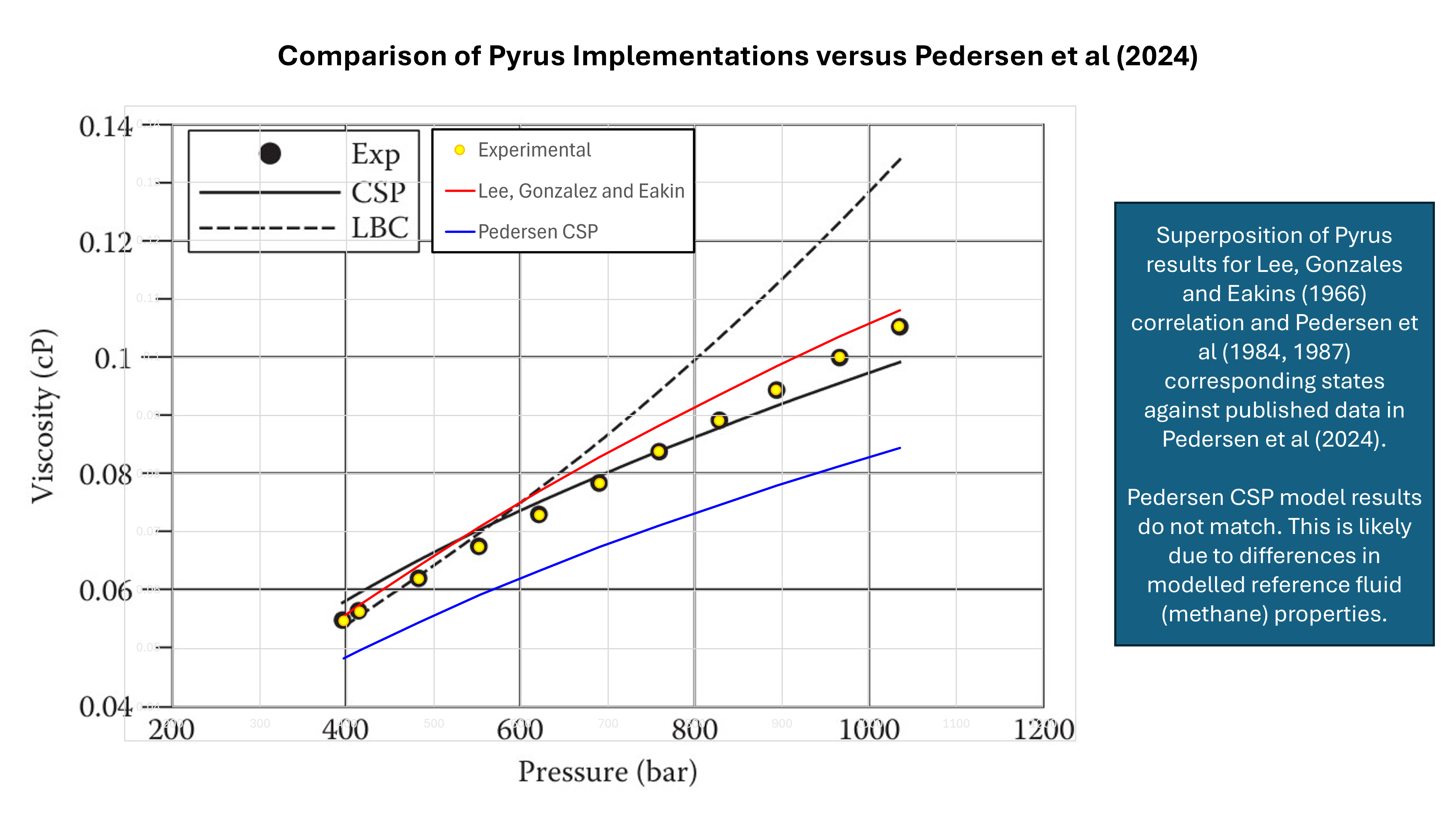
Comparison of the implemented method in Pyrus against the published data in Pedersen et al (2024) shows that there is a difference in the CSP results. Where Pedersen et al closely match the experimental data, the Pyrus implementation has a slightly lower viscosity. This shows that the method is sensitive to the reference fluid model used for the viscosity, density and critical point predictions.
In contrast, the Lee, Gonzalez and Eakin (1966) correlation which is often used in laboratories to provide a gas viscosity value in lieu of an experimental measurement, can be seen to be reasonably accurate. In testing it was also found that at higher pressures, the Pedersen CSP implementation could be very inaccurate for some pressure and temperature combinations. It is suspected this occurred due to the density of the reference fluid being in the liquid rather than vapour phase.
Due to these issues, which are probably related to my implementation of the method, rather than the method itself, the Pyrus implmentation of the Pedersen CSP is not currently exposed via the user interface.
References
- Hanley, H. J. M., McCarty, R. D., and Haynes, W. M. 1975. Equations for the Viscosity and Thermal Conductivity Coefficients of Methane. Cryogenics 15 (7): 413-417. https://doi.org/10.1016/0011-2275(75)90010-7.
- Lindeloff, N., Pedersen, K. S., Rønningsen, H.P., and Milter, J. 2003. The Corresponding States Viscosity Model Applied to Heavy Oil Systems. Paper presented at the Canadian International Petroleum Conference, Calgary, Alberta, Canada, 10-12 June. PETSOC-2003-150. https://doi.org/10.2118/2003-150.
- McCarty, R. D. 1974. A modified Benedict-Webb-Rubin Equation of State for Methane Using Recent Experimental Data. Cryogenics 14 (5): 276-280. https://doi.org/10.1016/0011-2275(74)90228-8.
- Pedersen, K. S., Christensen, P. L., and Shaikh, J. A. 2024. Phase Behavior of Petroleum Reservoir Fluids, third edition. Boca Raton: CRC Press.
- Pedersen, K. S., Fredenslund, A., Christensen, P. L., and Thomassen, P. 1984. Viscosity of Crude Oils. Chem Eng Sci 39 (6): 1011-1016. https://doi.org/10.1016/0009-2509(84)87009-8.
- Pedersen, K. S. and Fredenslund, A. 1987. An Improved Corresponding States Model for the Prediction of Oil and Gas Viscosities and Thermal Conductivities. Chem Eng Sci 42 (1): 182–186. https://doi.org/10.1016/0009-2509(87)80225-7.