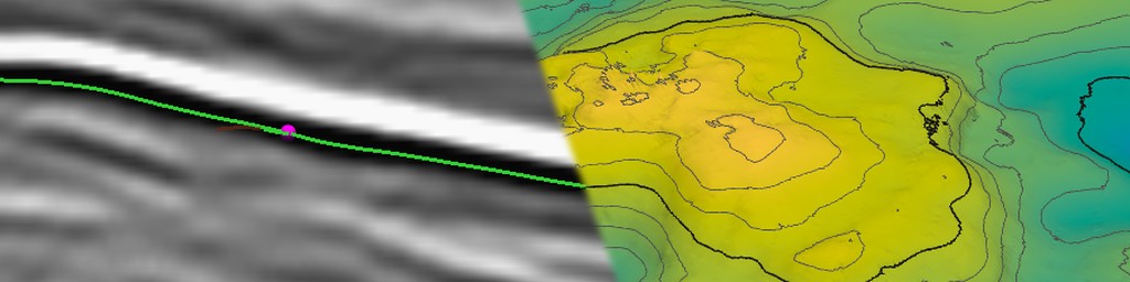
A seismic horizon emerges from the interpretation of a seismic volume where the objective is to identify where a reflection represents the same rock layers everywhere. Pick points that sit on similar layers across a few lines, join the dots, and voila, you have a map of the subsurface. In practice the dots refuse to join: the reflection fades, splits, crosses a fault and comes back a cycle higher or lower, and the software that was meant to follow it wanders off after a stronger neighbour. And whilst it is easy enough to see the lines that you have picked on 2D lines, doing the same in three dimensions is a little trickier. Not being a seismic interpreter myself, I was intrigued to see whether I could create a horizon interpretation technique in Pyrus. This would lead to the capability of building proper 3D grids, so from a simulation perspective it is an essential tool.
This post is part tutorial and part experiment. The tutorial half walks through interpreting a horizon in Pyrus from the first pick to a saved surface. The experiment half asks the obvious question: how close does the result come to an interpretation done properly, by the people who drilled the field?
For both, I’ve used Equinor’s Volve data set. Volve is a small oil field in the Norwegian North Sea that produced from 2008 until 2016, and in 2018 Equinor released essentially everything about it: seismic, wells, production data and, usefully for this post, the geophysical interpretations (Equinor, 2018). That makes it one of the very few places where you can compare your own horizon against a real one and publish the pictures.
The horizon is the Base Cretaceous Unconformity (BCU) which lies just above the Volve reservoir. It is one of the classic North Sea reflectors: regionally extensive, usually strong, and interpreted on almost every survey in the basin. It’s a fair test: easy enough that a tracker should cope, but with enough structure and changes in character to catch out a lazy one.
What Is a Horizon, Anyway?
To the software, a horizon is just a surface comprising a cloud of points that can be connected into a mesh: one two-way time (or depth) for each trace in the survey, \(z(x, y)\), sitting on the same inline/crossline lattice as the seismic. In Pyrus it is stored like every other surface, as a regular grid, so once it exists it can be coloured, contoured, exported and compared like any other surface.
The hard part is getting the numbers in the first place. An interpreter can see the reflection; the software has to be told what “the same reflection” means.
Why Not Just Follow the Peak?
The obvious approach is the one most of us learned first. Pick a point on a peak (or trough), step to the next trace, look a few samples up and down for the nearest peak, and repeat. It is simple, fast, and works beautifully right up until it doesn’t. The example shown in Figure 1 is illustrative based on the Parihaka 3D survey made available by New Zealand Petroleum and Minerals. It’s not a real picking algorithm (I just superimposed an indicative horizon pick on the image), but it clearly shows how an event encountering a fault can happily continue across a fault, seemingly oblivious to the presence of the fault.
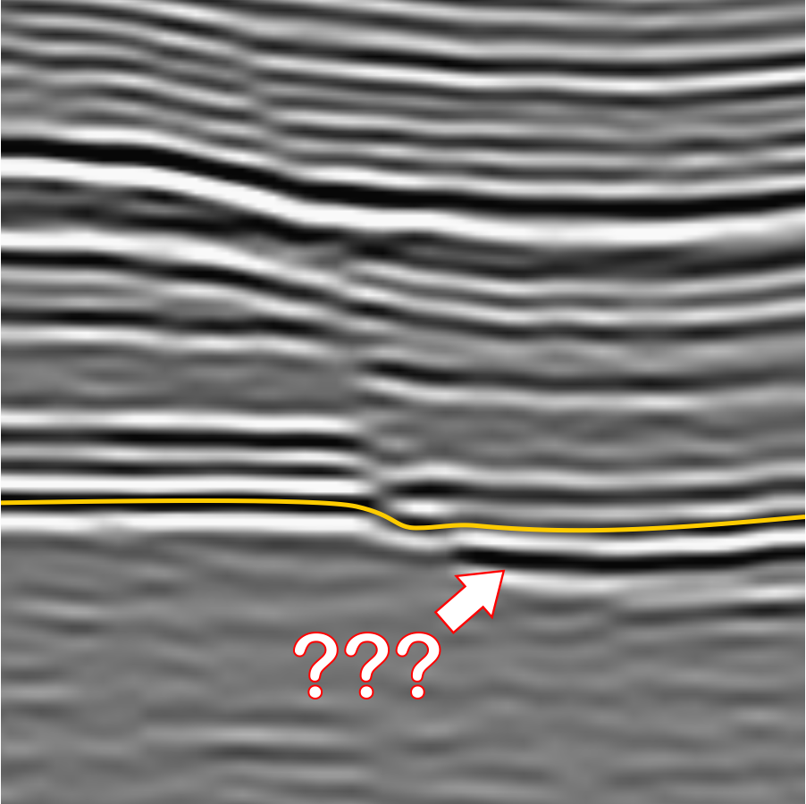
The trouble is that every decision is local and final. Once the tracker has stepped onto the wrong cycle, every later trace agrees with the mistake, because each one only compares itself with its neighbour. Errors don’t average out; they propagate. Faults, noise and places where the reflection dims are exactly where a human looks hardest and a peak-follower looks least.
What Works Better?
The method in Pyrus comes from Wu and Fomel (2018), who turned horizon picking from a sequence of local decisions into one global fit. Instead of asking “where is the peak on the next trace?”, it asks “which surface best agrees with the dip of the reflections everywhere, while passing through the interpreter’s picks?”
The first ingredient is the local slope of the reflections. At every sample of the seismic, a structure-tensor filter estimates how steeply the reflections dip in the inline and crossline directions, in samples per trace. A horizon that follows the reflections must have the same dip as the seismic at every point it passes through, which gives a pair of equations for each trace:
\[\frac{\partial z}{\partial x} = p(x, y, z), \qquad \frac{\partial z}{\partial y} = q(x, y, z)\]Where:
- z = horizon two-way time at trace (x, y) (samples)
- x, y = inline and crossline trace positions (traces)
- p, q = local reflection slopes in the inline and crossline directions, evaluated on the horizon (samples per trace)
There are far more equations than unknowns, and the slopes are noisy, so the horizon is found by least squares: the surface whose gradient matches the slopes as closely as possible, with the picks held fixed. Because the slopes themselves depend on where the surface is, the fit is iterated: evaluate the slopes on the current surface, solve, and repeat.
Slopes on their own have the same weakness as the peak-follower, only spread more evenly: integrate a small slope error over hundreds of traces and the surface drifts, and across a fault the slope says nothing useful at all. The second ingredient fixes this. Multigrid correlations cross-correlate traces that are not neighbours, but several traces apart on a series of coarser grids, and add the resulting time shifts as extra equations. These long-range links tie distant parts of the surface together directly, so they can bridge faults and stop slow drift.
Everything is solved together, so a doubtful patch is pulled into line by the good data around it instead of dragging everything after it off course. That is the essential difference from the peak-follower.
How Does Pyrus Do It?
Pyrus uses an adapted version of Xinming Wu’s open-source implementation, reworked to only read and load into memory the seismic from the HDF5 cube that is immediately needed for the algorithm. The brute force approach used loads the entire cube into memory, and then computes an additional three attribute cubes. So for a 25 GB cube, you’re very quickly reaching a memory requirement of 100 GB. Not outrageous, but still considerable even in 2026 when this post was written.
A horizon is built in three stages, each feeding the next:
- Picks. You click on the seismic to provide seed points that lie on the target horizon. Each pick is recorded against its inline, crossline and sample depth.
- Horizon lines. For each pick, the 2D version of the extractor (
HorizonExtractor2) tracks the horizon along the whole inline or crossline through it, and along any existing lines it intersects. These lines are what you see appear as you pick. The 2D horizon lines are used to build a crude mesh that forms the starting point for a 3D surface. - The surface. The 3D extractor (
HorizonExtractor3, or MHE3) fits the whole surface to the picks, starting from the simple surface generated from the 2D horizon line mesh.
The surface stage starts from an initial guess, and the quality of the guess matters. The original algorithm proposed by Wu, uses an initial surface that is set using radial basis function. This creates a smooth surface that interpolates between the points that have been picked. The downside of the approach is that it can wildly overshoot, which doesn’t necessarily prevent the algorithm from working, but it does massively increase the amount of work that needs to be done to find the best solution. Pyrus uses a completely different approach because of this. Inside the area covered by the picks, Pyrus uses Delaunay triangulation to build a triangulated irregular network (TIN) mesh from the picks and line samples, and then interpolates them with cubic Bézier patches built from Akima derivatives (Akima, 1970). Outside that area it uses a smooth biharmonic radial basis function, which extrapolates gently instead of wildly. The two are blended with a Gaussian weight on the distance from the convex hull of the picks. The blending loop is:
// Calculate convex hull that envelopes the picks.
List<double[]> hull = AdvMath.computeConvexHull2D(AdvMath.toXY(pcb.getAllPoints()));
float[][] hs_blend = new float[N3][N2];
double sigma = 20.0; // smoothing radius in samples
for (int i3 = 0; i3 < N3; i3++) {
    for (int i2 = 0; i2 < N2; i2++) {
        if (cancelled()) {
            return;
        }
        double x = i3 + i3lo;
        double y = i2 + i2lo;
        double d = AdvMath.hullPointDist(hull, new double[]{x, y});
        double w = Math.exp(-(d * d) / (sigma * sigma));

        // Blend generalised and RBF surfaces
        hs_blend[i3][i2] = (float) (w * hs[i3][i2] + (1.0 - w) * hs_rbf[i3][i2]);
    }
}
That blended surface is a quick preview that can be seem while picking. It is the starting surface that is provided to the MHE3 algorithm to produce a detailed surface. The starting point is then refined against the slopes and correlations. The slopes are computed lazily (meaning computed as and when needed by the algorithm, rather than pre-computing every possible slope and storing in a separate cube), only for the parts of the cube the solver actually visits, which keeps memory in check on large surveys:
LocalSlopeFinder lsf = new LocalSlopeFinder(horizon_sigma1, horizon_sigma2, horizon_sigma2, horizon_pmax);
LazySlopeVolume3D slopes = new LazySlopeVolume3D(vf, lsf);

// Initialise surface with seed point (this uses ROI coordinates).
HorizonExtractor3 he3 = new HorizonExtractor3();
he3.setSmoothings(horizon_smoothing, horizon_smoothing);
he3.setWeights(0.001f);
he3.setExternalIterations(10);
All of this runs as background tasks with generation counters, so you can keep picking while a surface is being computed, and a stale result never overwrites a newer one.
Interpreting the BCU on Volve, Step by Step
This is the practical part. The steps below are how I interpreted the BCU on Volve; the same steps apply to any horizon on any survey.
1. Load the Seismic
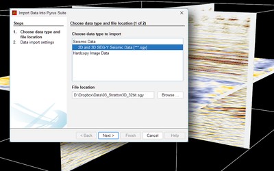
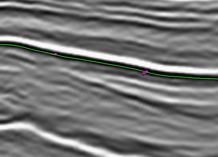
Load the Volve seismic cube in two-way time (Pyrus converts the SEG-Y to an HDF5 cube on first import, so later sessions open quickly). Set a vertical exaggeration that makes the reflections easy to follow; the vertical exaggeration or VE spinner in the editor panel goes from 1 to 10, and allows the vertical axis shown to be stretched. For this example we have loaded “ST0202R08_PZ_PSDM_FULL_OFFSET_PP_TIME.MIG_FIN.POST_STACK.3D.JS-017534.segy” which is the initial pre-discovery 3D pre-stack depth migrated seismic volume in time.
At the time this blog post was written, the only way to move the inline and crossline planes through the cube was with the arrow keys (LEFT / RIGHT for inlines, UP / DOWN for crosslines) and the time slice is similarly moved with PAGE UP> and PAGE DOWN. Before picking anything, scan through the survey and get a feel for where the BCU is strong, where it weakens and where the faults are. Five minutes spent looking saves an hour spent fixing. Note that different colour maps can be applied to the seismic which can aid with identification of the horizon during picking.
2. Start a New Horizon
Click Digitise Horizon to open the picking panel and enter horizon editing mode. Give the horizon a name in Horizon Information (I used “BCU (MHE3)”) and choose its line, marker and surface colours.
Under Pick Options, choose 2D Horizon Lines Only to pick on inlines and crosslines, or 2D Lines and 3D Points to allow picks on time slices as well. Start with lines only; time-slice picks are useful later to pin down awkward areas.
Note that for the first pick on a line, especially if the survey is very large, it may take a while to compute the local slopes along the line and show the picked line based on the seed point. The line is coloured solid green (as default; can be changed by user) in between actual picks on a line, and is coloured a semi-transparent dark red where the interpreted line is extrapolated outside the picked points. The green portions of the interpreted lines are used for generating the surfaces. The extrapolated lines are used to indicate the accuracy of where the algorithm would be likely to extend the surface.
3. Set the Autopick Constraints
The Autopick Horizon Constraints control how the slopes are measured and how smooth the surface is. The defaults suit most data, so I’d only change them once you’ve seen a result you don’t like.
| Control | Default | What it does | When to change it |
|---|---|---|---|
| Smoothing Half-Width: Down | 8 samples | Vertical extent of the window used to measure the reflection slopes | Increase for noisy data; decrease if thin, closely spaced reflections are being blurred together |
| Smoothing Half-Width: Across | 2 traces | Lateral extent of the same window | Increase on noisy data with gentle structure; keep small near faults |
| Maximum Slope | 3 samples/trace | Steepest dip the slope estimate will accept | Increase for steeply dipping horizons; the default is generous for most |
| Smoothing | 6 | How strongly the 3D surface is smoothed during the fit | Lower for more detail; higher for a calmer surface on noisy data |
| Trace Padding | 64 traces | How far the surface extends beyond the area covered by picks | Increase to extrapolate further; decrease to keep the surface close to the picks |
Symptoms and which control to adjust:
- Blurred thin beds: Reduce Smoothing Half-Width: Down (e.g., 4 samples)
- Jumping a cycle: Increase Maximum Slope or add manual picks where it occurs
- Surface too rough: Increase Smoothing
- Surface not reaching the survey edge: Increase Trace Padding
4. Pick a Few Lines
Click on the BCU on an inline. Pyrus records the pick and tracks the horizon along the whole line; the status bar shows the line, the world and cube coordinates and the two-way time of the pick. Check the tracked line from end to end. Where it strays, click on the correct reflection to add a pick there and the line is re-tracked through it. Shift-click a pick to delete it, and Undo (Ctrl + Z) reverses the last edit.
Then do the same on a crossline. A pick on one line also re-tracks the existing lines it crosses, so a sparse grid of lines quickly ties together. On Volve I picked seven inlines and seven crosslines, roughly evenly spaced apart. This is shown in Figure 3.
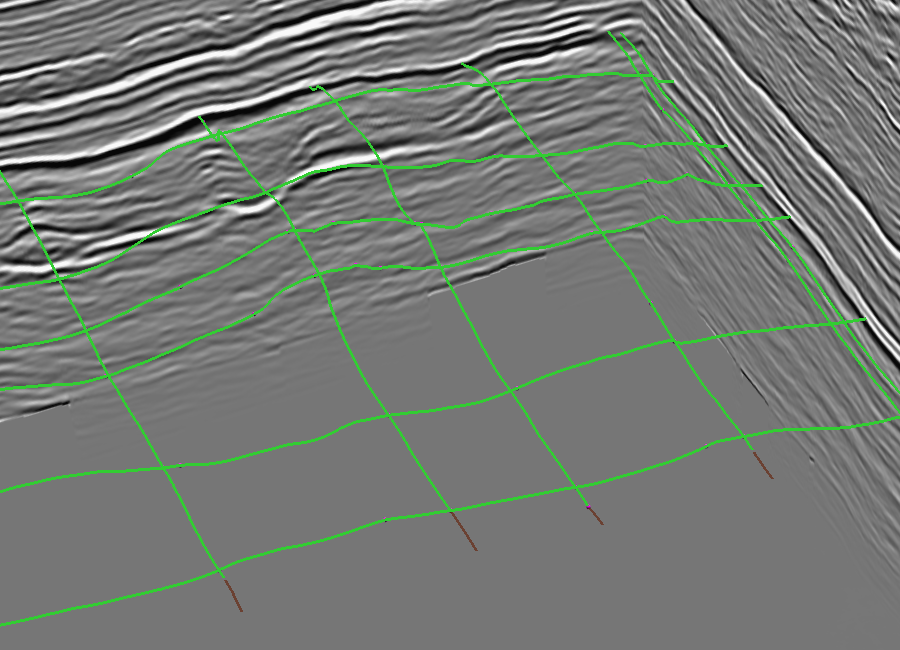
A few well-placed picks are worth more than many careless ones. The slopes do the heavy lifting between picks; your job is to tell the solver where the horizon is wherever the slopes alone can’t, mostly across faults and through dim patches.
The tool will automatically generate intersection picks when a crossline extends over an existing inline, and vice-versa. This can occasionally cause problems if the intersected line was not lying on the target horizon. It will be necessary to delete picks with Shift-click and repick them if this occurs. A useful strategy is to pick a range of only inlines or crosslines only before moving onto the intersecting lines. Depending on the quality and strength of the reflector being followed, this will not always be possible.
If picking of 3D points is enabled, then additional pick points for the horizon can be placed onto a slice. This allows for greater control of the final horizon.
5. Preview the Surface
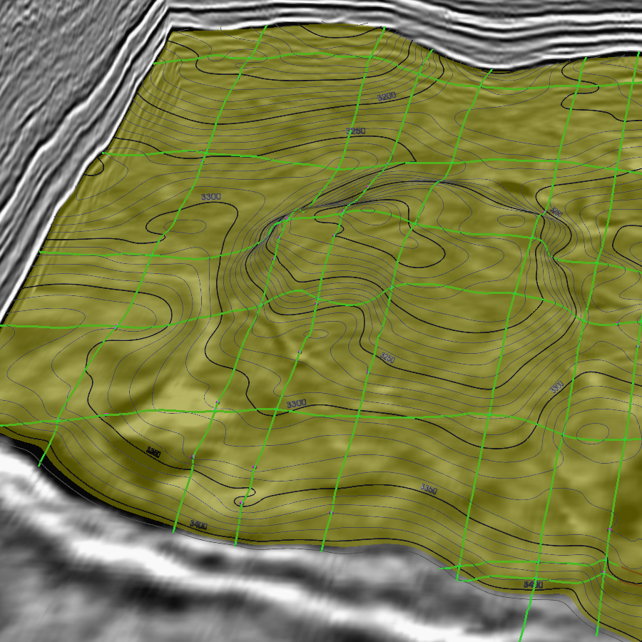
Tick Show surface to see the quick preview surface. It updates as you pick, and the Surface Opacity slider lets you see the seismic through it. The preview is good enough to spot gross errors, such as a line on the wrong cycle, which show up as a step or a fold in the surface. Picking ‘through’ the surface is possible provided it has some transparency.
6. Extract the Detailed Surface
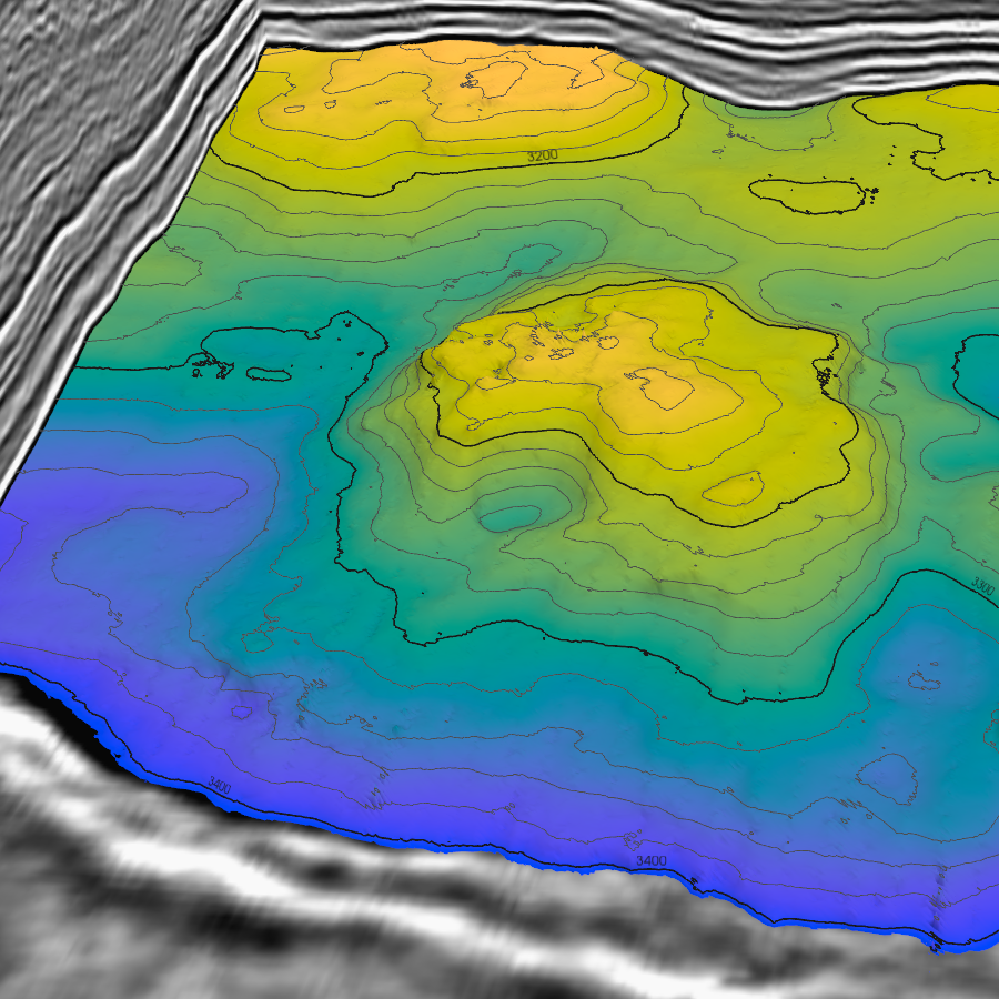
When the lines look right, click Extract 3D Horizon Surface. This runs the full MHE3 refinement over the picked area plus the trace padding. It takes considerably longer than the simple surface preview or the 2D interpreted lines; progress shows in the status bar, and the task can be cancelled. TODO: extraction time on Volve.
7. Check It
Quality control is the part that gets skipped, so it deserves its own step. Move the inline, crossline and time-slice planes through the surface and check that it sits on the reflection everywhere, not just near the picks. Contours help: tight, tangled contours usually mean the surface has jumped a cycle, and a straight contour running along a fault means the surface is smearing across it. Where you find a problem, add a pick there and extract again.
8. Save and Export
Click Save Horizon to save the surface into the project as a .vtkhdf file. It will appear in the project explorer as a horizon GeoObject. From then on it behaves like any other horizon: it can be coloured and contoured from the property sheet, and exported to ASCII XYZ (or other formats) by right-clicking on the object and selecting Export As…. Horizons can be exported as:
- .XYZ ASCII tab delimited format
- .zmap legacy ZMap+ format
- .vtu VTK surface format
- .csv comma separated values with ASCII text
More export formats are likely to be added in the future, such as GeoTIFF. Pyrus doesn’t aim to lock your data into the software. If you just want to interpret the horizons and then use them elsewhere, that’s a perfectly valid approach and is supported by Pyrus.
How Does It Compare With the Official Interpretation?
The Volve release includes Equinor’s own interpretation of the BCU. Theirs was done by interpreters who knew the field and had the wells, so it is the closest thing to a right answer available, though it is worth remembering that it is still an interpretation, not ground truth.
I imported it with the ASCII horizon importer in Pyrus, which works out the survey lattice from the points themselves. It can be seen that the offical horizon has small gaps in the corners which don’t extend to the very edge. Similarly the picks for the Pyrus version of the BCU appear to lose the horizon near the edges where there are no seed picks. Adding seed picks would undoubtedly help to resolve this issue.
With that fixed, the two surfaces can be overlaid. Setting both to partial opacity in the property sheet, in contrasting complimentary colours, makes the differences obvious. It can be seen that both surfaces are close to each other and no one surface dominates as higher than the other.
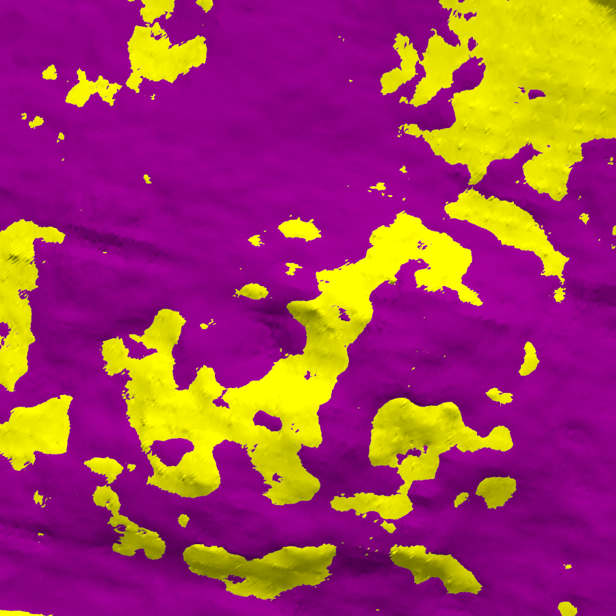
An overlay shows where the surfaces differ; numbers say by how much. Both horizons sit on the same survey lattice, so the comparison is simply the difference, MHE3 minus official, at every trace where both are defined:
\[\Delta t(x, y) = t_{\mathrm{MHE3}}(x, y) - t_{\mathrm{official}}(x, y)\]Where:
- Δt = time difference at trace (x, y) (ms)
- tMHE3 = two-way time of the MHE3 horizon (ms)
- tofficial = two-way time of the official horizon (ms)
Whilst this could potentially be done in the application, I simply exported both horizons as .csv and performed some statistical analyis in Excel. Sometimes the simplest brute force methods are the best. The summary statistics are:
| Measure | Value |
|---|---|
| Traces compared | 232,925 |
| Mean difference (bias) | −6 ms |
| Standard deviation | 87 ms |
| RMS difference | 87 ms |
| 10th percentile of |Δt| | −112 ms |
| 90th percentile of |Δt| | 141 ms |
| Within ±100 ms | 71 % |
| Largest difference | 218 ms |
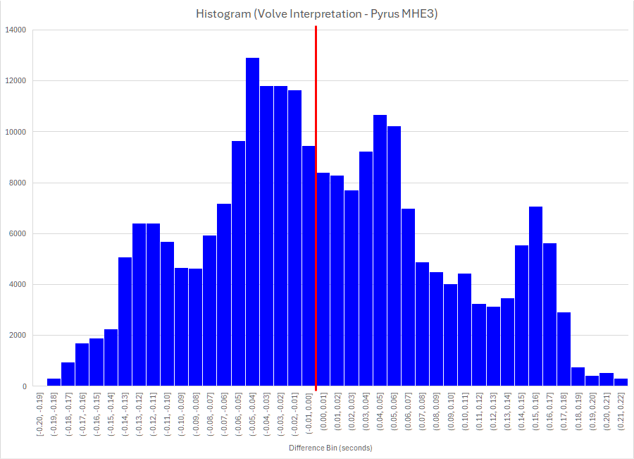
Clearly it’s not a perfect replication of the horizon. Is it reasonable? Well the mean difference of just −6 milliseconds suggests that there is very little bias in the picked horizons. That can also be easily seen in Figure 6 where sometimes the official interpreted horizon is higher, and at other points the Pyrus picked horizon is higher. There is no particular type of feature where one interpretation is weaker than the other, although the MHE3 horizon appears to struggle a little in areas where the event amplitude is very subdued (which is not too surprising).
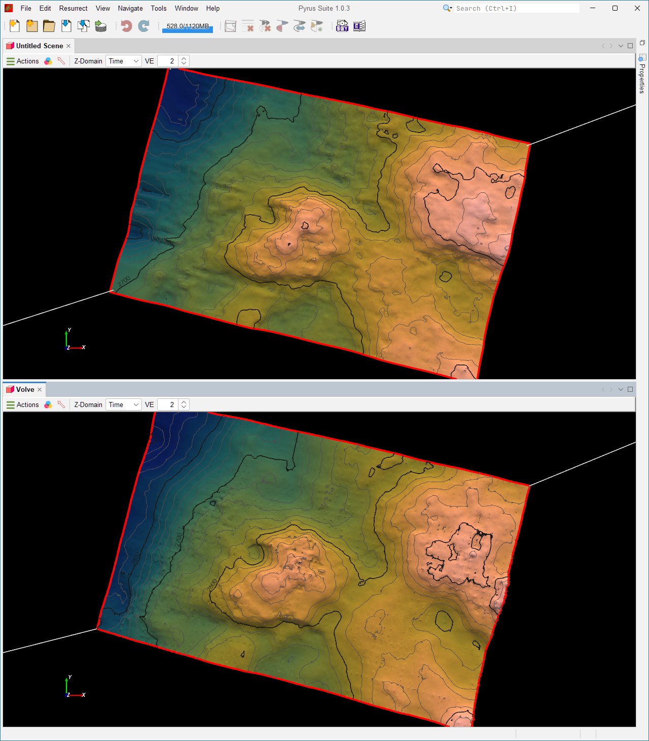
Another notable difference is that the geophysical interpretation from the Volve Data Village is much smoother. The MHE3 horizon has noticable noise and spikes/dimples that appear to align with the multigrid lattice that is overlaid on the horizon. No doubt this can be cleaned up and improved. A comparison between the two interpretations in Figure 8 shows that the overall shape and depths (in time) are the same. For the purposes of constructing a 3D simulation grid, this is more than sufficient as the noise inherent in the MHE3 interpretation would be smoothed out when building a static grid.
What Did I Learn?
Building my own seismic interpretation tool has taught me a few things about making seismic picks.
- With a suitable autopicking algorithm, it is not necessary to pick every single line to build a 3D horizon. The time saving is considerable. To pick the horizon shown here took about 15 minutes, and much of that time probably arises from my inexperience.
- A handful of picks in the right places (across faults, through dim zones) does more than many picks on easy ground.
- Solving for the whole surface at once is more forgiving than tracking trace by trace, because a bad patch is outvoted by the good data around it.
- Checking against someone the official interpretation shows that the result obtained by quickly picking a few lines and then letting the MHE3 algorithm run is nearly as good as the careful geophysical interpreter horizon.
The one-line lesson: let the seismic dips do the tracking, and spend your picks where the dips can’t be trusted.
Filling Gaps in a Horizon
Why Gaps Occur
Even with careful picking, horizons develop gaps. This happens when:
- Picks are too sparse - large distances between picks leave areas without constraints for MHE3 to fit to.
- Faults and complex structures - the gap filler cannot bridge across major discontinuities where no correlation exists.
- Noisy or dim data - if slopes can’t be measured reliably, the surface solver struggles in those regions.
Gaps appear as blank or empty space in the surface display where no interpolated value exists. They’re not errors; they’re honest representations of uncertainty. In other situations, imported horizons may not have been interpreted to the very edge of the cube. This causes problems for layered time to depth conversion, and it is necessary to extend the horizon surface so that layered velocity modelling becomes possible.
Running the Gap Filler
The gap filler runs automatically when you extract a detailed surface if gaps exist. However, you can also manually trigger it:
- With your horizon selected in the property sheet, click Fill Gaps (menu: Horizon > Fill Gaps, or toolbar button with the same label)
- The gap filler uses Akima interpolation to smooth across gaps that are smaller than a configurable threshold
- Progress shows in the status bar; larger surfaces may take 10-60 seconds depending on grid size
Options:
| Option | Default | What it does |
|---|---|---|
| Fill small gaps only | Yes (≤50 samples) | Don’t try to fill very large gaps that likely represent real structural breaks |
| Preserve edge picks | Yes | Never move picks at the survey boundary; this prevents artificial time shifts at edges |
Checking Filled Areas
After filling, verify the results:
- Visual inspection: Move inline and crossline planes through the filled area. The surface should follow reflections smoothly without obvious folds or jumps.
- Contour check: Look for tightly packed or tangled contours in filled regions - these indicate interpolation artifacts rather than real structure.
- Compare to seismic: Toggle between the horizon (partial opacity) and the underlying seismic. Filled areas should sit on consistent reflection peaks, not dim noise or multiple cycles.
If a filled area looks wrong, add more manual picks there and re-run extraction. The gap filler works best when you’ve provided enough constraints around problematic regions.
References
- Akima, H. 1970. A New Method of Interpolation and Smooth Curve Fitting Based on Local Procedures. J ACM 17 (4): 589-602. https://doi.org/10.1145/321607.321609.
- Equinor. 2018. Disclosing all Volve data. https://www.equinor.com/news/archive/14jun2018-disclosing-volve-data.
- Wu, X. and Fomel, S. 2018. Least-Squares Horizons With Local Slopes and Multigrid Correlations. Geophysics 83 (4): IM29-IM40. https://doi.org/10.1190/geo2017-0830.1.